
There are stories like this, the stories that remain in the backlog for a very long time, and finally, they get implemented. That's exactly what happened with the Dynamic Partition Pruning feature added, after almost 4 years in the backlog, to Apache Spark 3.
The blog post starts with the "why" and explains the reasons for implementing this feature. In the next part, you will learn about the configuration entries that are used in the algorithm that will be presented later. The article ends up with the physical execution, followed by a short demo showing what happens when the Dynamic Partition Pruning (DPP) is called in the query.
Why?
To understand why Dynamic Partition Pruning is important and what advantages it can bring to Apache Spark applications, let's take an example of a simple join involving partition columns:
SELECT t1.id, t2.part_column FROM table1 t1
JOIN table2 t2 ON t1.part_column = t2.part_column
At this stage, nothing really complicated. The query is a simple join that, depending on the size of the dataset, will transform or not into a broadcast join. But what happens if you add an extra WHERE clause to the query?
SELECT t1.id, t2.part_column FROM table1 t1
JOIN table2 t2 ON t1.part_column = t2.part_column
WHERE t2.id < 5
As you can deduce, the extra filtering condition identifies the partitions that should be kept on both sides of the join. In other words, the JOIN transforms into a simple SELECT ... WHERE:
SELECT t1.id, t1.part_column FROM table1 t1
WHERE t1.part_column IN (
SELECT t2.part_column FROM table2 t2
WHERE t2.id < 5
)
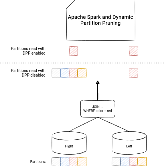
And that's the general idea behind the Dynamic Partition Pruning feature. How does it help Apache Spark process data more efficiently? The feature works on partitioned datasets and transforms one side of the join to a broadcasted "filter" used to skip the irrelevant partitions of another side of the join. They're irrelevant because of the "filter" result and hence reading them wouldn't generate any output rows.
Configuration
The configuration entries impacting the feature are prefixed with spark.sql.optimizer.dynamicPartitionPruning. The first of them is of course the enable/disable flag, added for a lot of new features in Apache Spark 3. When spark.sql.optimizer.dynamicPartitionPruning.enabled is set to true, which is the default, then the DPP will apply on the query, if the query itself is eligible (you will see that it's not always the case in the next section).
The second property is spark.sql.optimizer.dynamicPartitionPruning.reuseBroadcastOnly. It's another boolean flag controlling the use of the DPP. If this property is set to true (default), the DPP will apply only when the BroadcastExchange can be reused in the dynamic pruning filter. You should understand it a little bit better in the next section.
And finally, there are 2 properties responsible for the attributes used in the DPP. The spark.sql.optimizer.dynamicPartitionPruning.useStats, defines whether the distinct count of the join attribute should be used, and the spark.sql.optimizer.dynamicPartitionPruning.fallbackFilterRatio sets the fallback value to use in the algorithm when the stats are disabled or unavailable. Both have a crucial role in detecting whether yes or no, adding the pruning subquery will improve the query execution.
Algorithm
The logic for the DPP is included in the PartitionPruning logical optimization rule. In the entry point of this method you can already see that the DPP won't apply on the correlated subqueries and if the enable flag is set to false. For any other cases, it will try to add the pruning predicate:
    // Do not rewrite subqueries.
    case s: Subquery if s.correlated => plan
    case _ if !SQLConf.get.dynamicPartitionPruningEnabled => plan
    case _ => prune(plan)
What happens in the prune(LogicalPlan) method? First, it extracts "equi-join" keys, so the equality predicates used in the ON clause of the query. Later, it "flattens" the join condition predicates so that any conditions joined with AND are put at the same level, into a sequence. For example, an ON clause like "key1 = key2 AND key1 = key3" is transformed to an array of ["key1 = key2", "key1 = key3"].
If an equi-join condition is used on the columns coming from 2 different tables, the Dynamic Partition Pruning algorithm starts its work. First, it identifies the left and right columns for the join so that it can later apply its logic on one of them. First, it checks whether the DPP optimization can be used on the left side:
var partScan = getPartitionTableScan(l, left)
if (partScan.isDefined && canPruneLeft(joinType) &&
    hasPartitionPruningFilter(right)) {
  val hasBenefit = pruningHasBenefit(l, partScan.get, r, right)
  newLeft = insertPredicate(l, newLeft, r, right, rightKeys, hasBenefit)
}
The partScan variable indicates whether the join column is a partition column. The check is quite straightforward. It's a simple verification of the joined column on the schema (schema stores the partitioning specification). In case you wonder, there are no magic checks of "does the column from the left represent the same concept as the column from the right" thing. All this, it's the responsibility of the one who wrote the query. And since the join columns are supposed to represent the same things on different datasets, the simplicity makes sense.
Later, the canPruneLeft, checks if the join type is one of inner, left-semi or right outer. For the right side of the join executed just after the presented if statement, the canPruneRight returns true for inner and left outer types.
Finally, the last verification is made in hasPartitionPruningFilter(LogicalPlan). The implementation of this method is:
private def hasPartitionPruningFilter(plan: LogicalPlan): Boolean = {
  !plan.isStreaming && hasSelectivePredicate(plan)
}
The first part is quite clear, you can't apply DDP on the streaming applications. On the other hand, the second one is a little bit more mysterious since you have to know the definition of selective predicate. According to the code, a selective predicate is one for these conditions: LIKE, IN(...), binary comparison (==, <=, >=, <, >), or a string predicate (contains, ends with, starts with). And this check is run against the right side of the join (for left part resolution; against the left part for the right side resolution), which is important to highlight since so far all the verifications were made on the left side of the query (still, in the block processing left side of the query). You can see that for the validation part of the right join side:
partScan = getPartitionTableScan(r, right)
if (partScan.isDefined && canPruneRight(joinType) &&
    hasPartitionPruningFilter(left))
If you think that the dynamic predicate applies starting from now, it's not completely true. In fact, there is another condition, very important from the query performance point of view. It's executed inside a pruningHasBenefit( partExpr: Expression, partPlan: LogicalPlan, otherExpr: Expression, otherPlan: LogicalPlan) method:
// For the left side
val hasBenefit = pruningHasBenefit(l, partScan.get, r, right)
newLeft = insertPredicate(l, newLeft, r, right, rightKeys, hasBenefit)

// For the right side
val hasBenefit = pruningHasBenefit(r, partScan.get, l, left)
newRight = insertPredicate(r, newRight, l, left, leftKeys, hasBenefit)
In the hasBenefit, the engine checks whether applying the DPP would be more beneficial than leaving the query untouched. This is controlled with the following formula:
// the pruning overhead is the total size in bytes of all scan relations
val overhead = otherPlan.collectLeaves().map(_.stats.sizeInBytes).sum.toFloat

filterRatio * partPlan.stats.sizeInBytes.toFloat > overhead.toFloat
Let's suppose then that the right side of the join has 10MB of data and the filter ratio is the default fallback property introduced in the previous part of the blog post (0.5). For that configuration, if the left side of the join is greater than 20MB, then using the DPP will be considered as beneficial. The outcome of this verification is later used in the physical execution stage to know whether the DDP should be applied even if the broadcast exchange cannot be reused. In other words, it means that executing the subquery would be more efficient than leaving the plan in its initial form.
The fallback filter value is not used when the valid stats are available. If they do, the filterRatio will be computed as (1 - distinct values in the partitioning column on the right side / distinct values in the partitioning column on the left side) [opposite for the right side check]:
val partDistinctCount = distinctCounts(leftAttr, partPlan)
val otherDistinctCount = distinctCounts(rightAttr, otherPlan)
val availableStats = partDistinctCount.isDefined && partDistinctCount.get > 0 &&
  otherDistinctCount.isDefined
if (!availableStats) {
  fallbackRatio
} else if (partDistinctCount.get.toDouble <= otherDistinctCount.get.toDouble) {
  // there is likely an estimation error, so we fallback
  fallbackRatio
} else {
  1 - otherDistinctCount.get.toDouble / partDistinctCount.get.toDouble
}
Once all lights are green, the DPP is added to the plan but only when it's worth or spark.sql.exchange.reuse is enabled:
val reuseEnabled = SQLConf.get.exchangeReuseEnabled
val index = joinKeys.indexOf(filteringKey)
if (hasBenefit || reuseEnabled) {
  // insert a DynamicPruning wrapper to identify the subquery during query planning
  Filter(
    DynamicPruningSubquery(
      pruningKey,
      filteringPlan,
      joinKeys,
      index,
      !hasBenefit || SQLConf.get.dynamicPartitionPruningReuseBroadcastOnly),
    pruningPlan)
} else {
  // abort dynamic partition pruning
  pruningPlan
}
Physical execution
As you can see, a new node DynamicPruningSubquery is then added to the query plan. It has an interesting flag represented by !hasBenefit || SQLConf.get.dynamicPartitionPruningReuseBroadcastOnly expression, that can invalidate the optimization at runtime. This expression is assigned to a property called onlyInBroadcast. If it's set to true and there is no chance to reuse the BroadcastExchange (reuse == no recomputation), the execution ignores the dynamic pruning by adding this dummy node always evaluated to true:
// PlanDynamicPruningFilters (physical planner)
val canReuseExchange = SQLConf.get.exchangeReuseEnabled && buildKeys.nonEmpty &&
          plan.find {
            case BroadcastHashJoinExec(_, _, _, BuildLeft, _, left, _) =>
              left.sameResult(sparkPlan)
            case BroadcastHashJoinExec(_, _, _, BuildRight, _, _, right) =>
              right.sameResult(sparkPlan)
            case _ => false
          }.isDefined

        if (canReuseExchange) {
// ...
          DynamicPruningExpression(InSubqueryExec(value, broadcastValues, exprId))
        } else if (onlyInBroadcast) {
          // it is not worthwhile to execute the query, so we fall-back to a true literal
          DynamicPruningExpression(Literal.TrueLiteral)
In the least resort, so when the engine can't reuse the broadcast but executing the subquery is cheaper than leaving the plan untouched (cf. the filter ratio-based comparison), this check adds the subquery node (onlyInBroadcast is false):
          // we need to apply an aggregate on the buildPlan in order to be column pruned
          val alias = Alias(buildKeys(broadcastKeyIndex), buildKeys(broadcastKeyIndex).toString)()
          val aggregate = Aggregate(Seq(alias), Seq(alias), buildPlan)
          DynamicPruningExpression(expressions.InSubquery(
            Seq(value), ListQuery(aggregate, childOutputs = aggregate.output)))
        }
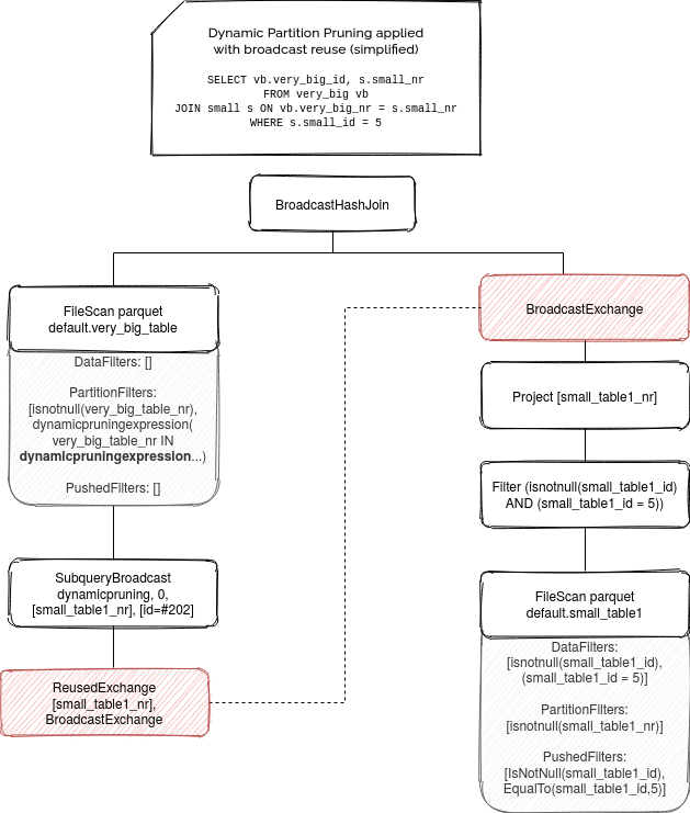
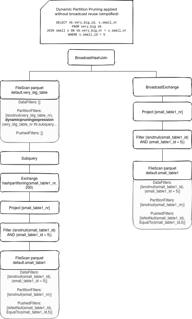
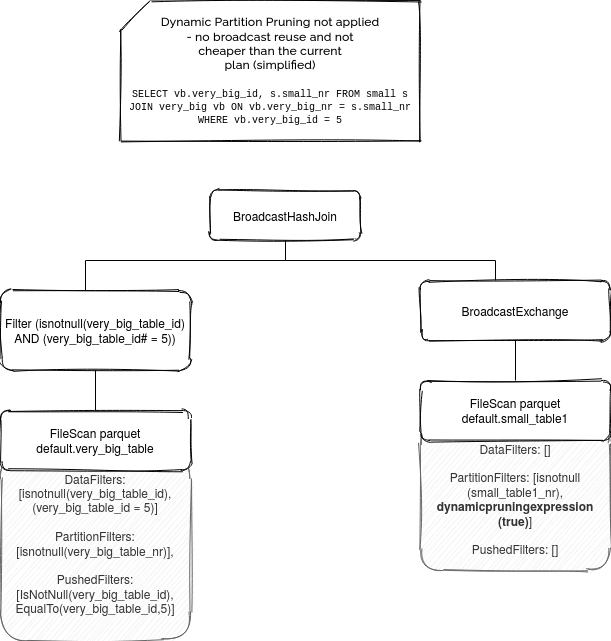
You can see all these 3 plans in the following simplified ASTs:
Before terminating, let's see how all these examples work on real queries:
The Dynamic Partitioning Pruning is then another great feature optimizing query execution in Apache Spark 3.0. Even though it's not implemented yet with the Adaptive Query Execution covered some weeks ago, it's still a good opportunity to make the queries more adapted to the real data workloads.