
In October I published the post about Partitioning in Spark. It was an introduction to the partitioning part, mainly focused on basic information, as partitioners and partitioning transformations (coalesce and repartition). This time it's a good moment to take other partition points up.
What would it take for you to trust your Databricks pipelines in production?
A 3-day bug hunt on a 3-person team costs up to €7,200 in lost engineering time. This workshop teaches you to prevent that — unit tests, data tests, and integration tests for PySpark and Databricks Lakeflow, including Spark Declarative Pipelines.

Konieczny
This post focuses mainly on 3 things. The first one presented in the first section talks about choosing the correct number of partitions and potential problems of bad partitioning. The second part shows how Spark loads data and distributes it to the executors. Finally, the last part presents the tests with partitions number.
Choosing the good number of partitions
A correct number of partitions influences application performances. After all, partitions are the level of parallelism in Spark. Bad balance can lead to 2 different situations. Too many small partitions can drastically influence the cost of scheduling. It means that the executor will pass much more time on waiting the tasks. In the other side, when there are too few partitions, the GC pressure can increase and the execution time of tasks can be slower. Moreover, too few partitions introduce less concurrency in the application.
So how to chose the good number of partitions ? During Spark Summit 2014, Aaron Davidson gave some tips about partitions tuning. He also defined a reasonable number of partitions resumed to below 3 points:
- commonly between 100 and 10000 partitions (note: two below points are more reliable because the "commonly" depends here on the sizes of dataset and the cluster)
- lower bound = at least 2*the number of cores in the cluster
- upper bound = task must finish within 100 ms
The number of calculated partitions defines the number of tasks in the last RDD in the stage. However, this number can change when the transformations as coalesce or repartition are called. To remind, the first one creates RDD with fewer partitions while the second increases or decreases the number of partitions.
Partition data distribution
Partition level can be defined on reading data from external sources. But what happens when Spark, for instance, reads a file from HDFS or receives new messages from Kafka ?
The case of Hadoop files is straightforward. During the generation of HadoopRDD, Spark defines the minimal number of partitions for the file. But in fact each partition corresponds to HDFS file split . Thus Spark uses already existent mechanism to partition HDFS data. The same logic applies to binary files (org.apache.spark.SparkContext#binaryFiles(path: String, minPartitions: Int ). The only difference is underlyed Hadoop's InputFormat (CombineFileInputFormat implementation instead of TextInputFormat).
HDFS file split
Basically, HDFS files are stored in blocks. The blocks are considered as physical representation. For map stage from MapReduce, each block contains a subset of data called split. But the splits can overlap and one block can contain the beginning of some content and the next block the rest of it. This aspect is considered as logical representation and is mainly used during processing. The following image shows that much better:
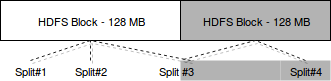
These chunks are processed later by MapReduce algorithm.
Please note that the parameter in binaryFiles and textFiles methods is the minimal number of partitions. Thus it's only a hint to Spark about the number of partitions. Often (most of time for HDFS files?) Spark will choose other numer of final partitions.
Regarding to DStream streaming, for instance Kafka DStream, Spark also uses the logic provided by datasource. In this case, each RDD partition corresponds to the pair of Kafka's topic-partition. For the case of Receiver-based processing, the number of partitions is equal to the result of batch interval / block creation interval size. For instance, if the streaming micro batch is of 10 seconds and the blocks are created every 500 ms, a RDD with 20 partitions will be created. However, by default all partitions will be stored on a single node holding the instance of receiver creating given block. Thus to improve the performances and balance the workload, it's recommended to create several receivers and use DStream's union(that: DStream[T]) operation allowing to process all received data in parallel.
Choosing the good number of partitions examples
To see what happens if there too many or too few partitions, we'll execute a micro-benchmark. The test assertions correspond to the results generated on my Lenovo Core i3 laptop having 4 cores. The results can vary in other environments:
val conf = new SparkConf().setAppName("Spark partitions micro-benchmark").setMaster("local[*]")
val sparkContext = new SparkContext(conf)

after {
  sparkContext.stop()
}

"the optimal number of partitions" should "make processing faster than too few partitions" in {
  val resultsMap = mutable.HashMap[Int, Map[Int, Long]]()

  for (run <- 1 to 15) {
    val executionTime1Partition = executeAndMeasureFiltering(1)
    val executionTime6Partition = executeAndMeasureFiltering(6)
    val executionTime8Partition = executeAndMeasureFiltering(8)
    val executionTime25Partition = executeAndMeasureFiltering(25)
    val executionTime50Partition = executeAndMeasureFiltering(50)
    val executionTime100Partition = executeAndMeasureFiltering(100)
    val executionTime500Partition = executeAndMeasureFiltering(500)
    if (run > 5) {
      val executionTimes = Map(
        1 -> executionTime1Partition, 6 -> executionTime6Partition, 8 -> executionTime8Partition,
        25 -> executionTime25Partition, 50 -> executionTime50Partition, 100 -> executionTime100Partition,
        500 -> executionTime500Partition
      )
      resultsMap.put(run, executionTimes)
    }
  }

  val points = Seq(7, 6, 5, 4, 3, 2, 1)
  val pointsPerPartitions = mutable.HashMap(1 -> 0, 6 -> 0, 8 -> 0, 25 -> 0, 50 -> 0, 100 -> 0, 500 -> 0)
  val totalExecutionTimes = mutable.HashMap(1 -> 0L, 6 -> 0L, 8 -> 0L, 25 -> 0L, 50 -> 0L, 100 -> 0L, 500 -> 0L)
  for (resultIndex <- 6 to 15) {
    val executionTimes = resultsMap(resultIndex)
    val sortedExecutionTimes = ListMap(executionTimes.toSeq.sortBy(_._2):_*)
    val pointsIterator = points.iterator
    sortedExecutionTimes.foreach(entry => {
      val newtPoints = pointsPerPartitions(entry._1) + pointsIterator.next()
      pointsPerPartitions.put(entry._1, newtPoints)
      val newTotalExecutionTime = totalExecutionTimes(entry._1) + entry._2
      totalExecutionTimes.put(entry._1, newTotalExecutionTime)
    })
  }

  // The results for 6 and 8 partitions are similar;
  // Sometimes 6 partitions can globally perform better than 8, sometimes it's the contrary
  // It's why we only make an assumptions on other number of partitions
  pointsPerPartitions(8) should be > pointsPerPartitions(1)
  pointsPerPartitions(8) should be > pointsPerPartitions(25)
  pointsPerPartitions(6) should be > pointsPerPartitions(25)
  pointsPerPartitions(8) should be > pointsPerPartitions(50)
  pointsPerPartitions(8) should be > pointsPerPartitions(100)
  pointsPerPartitions(8) should be > pointsPerPartitions(500)
  // The assumptions below show that, unlike primitive thought we'd have, more partitions
  // doesn't necessarily mean better results. They show that the task and results distribution overheads
  // also have their importance for job's performance
  pointsPerPartitions(25) should be > pointsPerPartitions(50)
  pointsPerPartitions(50) should be > pointsPerPartitions(100)
  pointsPerPartitions(100) should be > pointsPerPartitions(500)
  // Surprisingly, the sequential computation (1 partition) is faster than the distributed and unbalanced
  // computation
  pointsPerPartitions(1) should be > pointsPerPartitions(500)
  // Below print is only for debugging purposes
  totalExecutionTimes.foreach(entry => {
    val avgExecutionTime = entry._2.toDouble/10d
    println(s"Avg execution time for ${entry._1} partition(s) = ${avgExecutionTime} ms")
  })
}

private def executeAndMeasureFiltering(partitionsNumber: Int): Long = {
  var executionTime = 0L
  val data = sparkContext.parallelize(1 to 10000000, partitionsNumber)

  val startTime = System.currentTimeMillis()
  val evenNumbers = data.filter(nr => nr%2 == 0)
    .count()
  val stopTime = System.currentTimeMillis()
  executionTime = stopTime - startTime
  executionTime
}
Through this post we could learn about choosing the right number of partitions. The first part gave the response to the question about how many partitions should be generated. As we could see, the formula used to calculate this number was 2*number of cores in the cluster. The second part shown however that the number of partitions can be related to datasource. We saw 2 cases - HDFS files and Kafka topics, that were partitioned according to, respectively, file splits and topic-partitions pairs. The last part proved that the balanced number of partitions helped Spark to perform better than the unbalanced.
Data Engineering Design Patterns

Looking for a book that defines and solves most common data engineering problems? I wrote
one on that topic! You can read it online
on the O'Reilly platform,
or get a print copy on Amazon.
I also help solve your data engineering problems contact@waitingforcode.com 📩
Read also about Partitioning internals in Spark here:
- Input Splits in Hadoop's MapReduce Hadoop input split size vs block size RDD partitioning in spark Streaming
Related blog posts:
- Sacks - data parallelization unit in Gnocchi
- Data partitioning in Apache Beam
- Partitioning RDBMS data in Spark SQL
- Partitioning in Spark