
Some time ago I covered in this blog the complexity of Scala immutable collections, explaining a little what happened under-the-hood. Now it's a good moment to back to this topic and apply it for mutable collections.
Data Engineering Design Patterns

Looking for a book that defines and solves most common data engineering problems? I wrote
one on that topic! You can read it online
on the O'Reilly platform,
or get a print copy on Amazon.
I also help solve your data engineering problems 👉 contact@waitingforcode.com 📩
This post, like the one about Collections complexity in Scala - immutable collections, will be divided in the sections dedicated to each type of mutable collection. Some of them, apart of operations complexity explanation, will contain also the notes about implementation details. At the end the complexity of all described collections will be summarized in a comparison table.
Buffers
The first category of mutable collections represents buffers. ArrayBuffer is one of buffer's implementations and as its name indicates, it's backed by an array. The array has a predefined size that it specified during the class instance construction. Thanks to the array this kind of buffer is pretty efficient for the random access and write operations (constant time O(1)).
However, as in the case of Java's ArrayList, the underlying array can sometimes be resized in the case of append. Thus the complexity of this operation is amortized constant time (read more about Amortized and effective constant time). The similar rule applies for prepend operation. Here the content of the array is shifted one position to the right (thus the array is resized +1) and a new element is inserted at the 1st position (O(n) complexity).
Another implementation of mutable buffer is ListBuffer. Unlike ArrayBuffer it's backed by a linked list. Since the linked list is composed of nodes where each of them is linked to the next one with a pointer, it guarantees constant time prepend and append operations. But in the other side, it takes linear complexity (O(n)) for random access operations.
Array-related
The next category concerns arrays. Among the mutable collections related to the arrays we can distinguish 3 major ones: Array, ArraySeq and ArrayStack. The first of them and at the same time the most basic, Array, is mutable and indexed sequence of values backed by an array. That said, it's Scala's representation of Java's T[] array. It's good suited for primitive types since there is no overhead for boxing and unboxing operations. It means that Scala's Array[Int] is equal to Java's int[]. Array benefits from all Scala's sequence features thanks to the implicit conversion to an instance of WrappedArray. The test below shows that pretty clearly:
val arrayNumbers = new Array[Int](3)
val arraySequence: Seq[Int] = arrayNumbers

arraySequence shouldBe a [mutable.WrappedArray[_]]
The array is constant time for index-based operations (get and put) since it has a fixed size and can't be resized automatically.
The ArraySeq is a collection backed by an array of objects. This fact guarantees the constant execution time for the in-place modifications (since the direct access by index). Initially, because ArraySeq has a Seq in its name, we could think that every index out of bounds would lead to the array resizing. However it's not the case and instead an IndexOutOfBoundsException is thrown. So, what is the difference between ArraySeq and an Array ? The biggest one comes from the perception of stored elements. ArraySeq stores objects in a Java's plain array and that even if the elements are primitives. Array, as already told, stores primitive types as it, so without boxing and unboxing. But in terms of time complexity, Array and ArraySeq share the same characteristics.
The last array-like mutable collection is ArrayStack - a LIFO stack. As indicated by the name, it's backed by an array, thus benefits from random access and writes constant time execution the operation based on indexes (get, update). But since it's also a stack, it implements the operations like pop (gets last element of the array) and push (adds the element at the end of the array). And the latter one is amortized constant time because of the risk of array automatic resizing if it doesn't have any free indexes to handle new elements.
ArrayBuffer could also included in this list but it was already covered in the part about buffers.
Set
The set is a data structure without duplicates. In Scala we can find its 4 main implementations: HashSet, TreeSet, LinkedHashSet and BitSet. The first of them, HashSet is backed by an array of size 32 (table: Array[AnyRef]). As you can automatically deduce from the previous collections, adding new elements is not purely constant time since sometimes the underlying array may need some resizing. In such case, a new array, twice bigger as the initial one, is created and the entries from the old array are copied to it. Another specificity of the HashSet is the fact that it uses a hash table. When a new element is added, the hash code of the added element is computed. So computed value is used to determine the index of the element in the hash table. If there is no element at given place and the array doesn't need resizing, this operation takes constant time. Otherwise, it takes effective constant time either because of the resizing or/and of the potential hash collision (a new index is searched for the added entry in this case). The hash table also guarantees a fast (effective O(1)) execution of contains operation since it's a simple lookup in the underlying array. It's effective because of the collisions that are resolved in the same manner as the adds. The add logic is represented in the following snippet from FlashHashTable:
protected def addEntry(newEntry : AnyRef) : Boolean = {
  var h = index(newEntry.hashCode)
  var curEntry = table(h)
  while (null != curEntry) {
    if (curEntry == newEntry) return false
    h = (h + 1) % table.length
    curEntry = table(h)
    //Statistics.collisions += 1
  }
  table(h) = newEntry
  tableSize = tableSize + 1
  nnSizeMapAdd(h)
  if (tableSize >= threshold) growTable()
  true

}
Another common set type is TreeSet. It's backed by a data structure called red-black tree. One of its characteristics tells that the max height of it is 2 * log(n + 1) where n is the number of nodes. Since this kind of tree is self balancing and binary search tree, this property guarantees logaritmic complexity for insert, delete and lookups .
Red-black tree
The red-black tree is a binary search, self-balancing tree which nodes are labeled either black or red. The self-balancing property keeps the height of the tree as small as possible. The following image shows how an unbalanced tree became balanced:

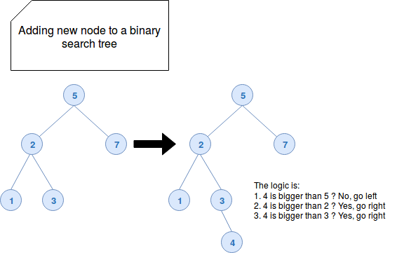
The binary search character of the tree helps to keep the nodes in a particular order: smaller values are located on the left part, bigger on the right side. The logic is shown in the following picture:
The red-black tree also has its specific requirements:
- every node is black or red
- root node is always black
- 2 adjacent nodes don't exist (red color nodes can't have red color parent nodes)
- every path from root to a NULL node has same number of black nodes
- every NULL node is always black
Every time when one of them is broken, either with a recently added node or a removed node, the tree is rebalanced. And finally it brings the O(log(n)) complexity for: adds, removals and lookups.
LinkedHashSet is another mutable set type available in Scala. At first glance we could think that it's backed by a linked list. However it's not the case because the underlying data structure is, as in the case of HashSet, an array. But unlike HashSet, this array is composed of HashEntry[A, Entry] instances. Another specificity of the LinkedHashSet is that it iterates over the elements in order of insertion. This behavior is guaranteed by the properties called earlier and later of the HashEntry object. These properties guarantee effective constant time execution for add operation because of eventual risk of underlying hash table resizing and collisions. Random access operations able to use the array as contains are also executed in effective O(1) for the same reasons.
The last set type is BitSet. This data structure stores ints as 64-bits "words" in an array that can be dynamically resized if the size is too small regarding to the number of added elements. Because of that the complexity of insert operation automatically becomes amortized. The array guarantees also purely constant time execution for random access operations as get/contains (both have the same meaning). The mutable version of BitSet is slightly more efficient for update operation because it doesn't have to copy around Longs that haven't changed.
Map
Scala has a wide choice of maps. Except well known TreeMap and HashMap, it proposes other less common ones: LinkedHasMap, ListMap, OpenHashMap, LongMap and other. Here we'll focus on the maps listed above. Let's begin with TreeMap. As in the case of the TreeSet it uses the red-black tree as the backed structure keeping the elements. So exactly as in the case of its set's cousin, TreeMap takes logarithmic time to search, remove and add operations. Similarly, the specificity for HashMap are the same as the ones of HashSet since it also uses hash table as the underlying structure. The search, add and remove operations are executed in effective constant time. The performance varies depending on fact if there is already a value for given hash or not. HashMap uses closed addressing and thus if a hash collision happens, the entry already defined in the hash table is added to the new entry as a pointer inside next attribute. Let's take the example from the following snippet:
class ConflictingClass(val name: String) {
  override def equals(obj: scala.Any): Boolean = false
  override def hashCode(): Int = name(0).toInt
  override def toString: String = name
}

val mapOfConflictingObjects = new scala.collection.mutable.HashMap[ConflictingClass, Int]()
val conflicting1 = new ConflictingClass("1abc")
val conflicting2 = new ConflictingClass("1def")
val conflicting3 = new ConflictingClass("2ghi")
mapOfConflictingObjects.put(conflicting1, 1)
mapOfConflictingObjects.put(conflicting2, 2)
mapOfConflictingObjects.put(conflicting3, 3)

println(s"Map=${mapOfConflictingObjects}")
// It will print: Map=Map(2ghi -> 3, 1def -> 2, 1abc -> 1)
The closed addressing is shown in the following capture, taken at the moment where conflicting object is added t to the map (so conflicting1 is already present there):

LinkedHashMap also uses hash table to store the elements. It benefits of the O(1) complexity for get or contains operations. However unlike HashMap it guarantees the order of iteration corresponding to the order of insertion. It's provided by scala.collection.mutable.LinkedEntry and its 2 properties: earlier and later.
Another map letting the insertion-order iteration is ListMap. The data is backed by a list storing tuples composed of key and value (key, value). As you can immediately deduce, the complexity for random access operations is linear (O(n)). The elements are prepended to the list, i.e. the newest keys are at the head. of the list thus getting the head is also O(n) while retrieving the last added item is O(1). The O(n) complexity applies also for the last method returning the last item in the map. The head operation executes in contant time since the ListMap uses IterableLike.head method calling the first element of the iterator:
override /*TraversableLike*/ def head: A = iterator.next()
The next of available maps, OpenHashMap. As in HashMap the entries are also stored in a hash table but they're wrapped in OpenEntry class storing: key, value and hash for given cell. Since the table can be automatically resized if needed, the complexity of add operation is effective. The lookup operation is effective constant time since it relies on a well hash key distribution that shows the following implementation:
def get(key : Key) : Option[Value] = {
  val hash = hashOf(key)
  var index = hash & mask
  var entry = table(index)
  var j = 0
  while(entry != null){
    if (entry.hash == hash &&
        entry.key == key){
      return entry.value
    }

    j += 1
    index = (index + j) & mask
    entry = table(index)
  }
  None
}
As you can see, the entry could be "misplaced" because of bad hash distribution and the get method can sometimes do multiple hash table lookups. This hashing addressing is called open (hence OpenHashMap). In the case of a collision this strategy looks for the first available cell to put there a value. This implementation is similar to the one of Python dictionaries.
The last map to cover is LongMap. It's a specialized map with keys of Long type. The keys and values are stored in 2 separate arrays. Even though the complexity is similar to the one of HashMap, LongMap (and its variance AnyRefMap) is supposed to be faster on the operation on single entities as contains or get, mostly thanks to this specialization. As you can deduce, the LongMap is also impacted by an operation called repacking that improves the performance underlying array but sometimes may slow down another operation. It's executed together with update method.
Queue
Among the queues (First-in First-out [FIFO] semantic) we can distinguish Queue and PriorityQueue. The former one is the simplest version of this data structure. The data is stored in a list so naturally all random access operations (get and update) are O(n) complexity. In the other side, the complexity for enqueue (append) and dequeue (head) is O(1).
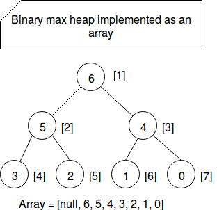
A more complex queue is PriorityQueue. It's a queue using binary max heap where the entries with the biggest values are stored on the beginning of underlying array. And who tells an array, he tells resizing and thus amortized constant time for add operation. However this complexity doesn't apply to PriorityQueue that, in addition to inserting given entry to the array, must sometimes do some reordering to satisfy the heap property telling that the value of parent node must be always greater than or equal to the value of both children. Thus, the complexity for this case is logarithmic (O(log n)). In the other side, since the entries are ordered, getting the first (= the most important) element is O(1). The following image shows how Scala translated the binary heap, that is a tree, to an array and how it manages the links between parent and children nodes:
Stack
The stack is a data structure following Last-in First-out (LIFO) semantic. The deprecated version of mutable Stack won't be explained in this section. However it exists another stack-type, ArrayStack that is still supported. Backed by an array, it performs pretty good for pop (stack's synonym of head), random access get and update operations (O(1)). It performs a little bit worse for push (prepend) one where the underlying array may sometimes need to be resized and thus the complexity becomes amortized constant time.
Complexity table
After describing some main mutable sequences, it's time to resume their complexities in the table below. The table is similar to the one from Collections Performance Characteristics. The difference is that it: is expressed in Big O notation, doesn't have the complexity for head and tail operation since they're always, respectively, constant and linear time, and has some supplementary sequences:
| Sequence | access per index | update | prepend | append | |
|---|---|---|---|---|---|
| ArrayBuffer | O(1) | O(1) | O(n) | a.O(1) | |
| ListBuffer | O(n) | O(n)O(1) | O(1) | ||
| Array | O(1) | O(1) | - | - | |
| ArraySeq | O(1) | O(1) | - | - | |
| ArrayStack | O(1) | O(1) | a.O(1) | O(n) | |
| HashSet | e.O(1) | e.O(1) | - | - | |
| TreeSet | O(log n) | O(log n) | - | ||
| LinkedHashSet | e.O(1) | e.O(1) | - | - | |
| BitSet | O(1) | a.O(1) | - | - | |
| HashMap | e.O(1) | e.O(1) | - | - | |
| TreeMap | O(log n) | O(log n) | - | - | |
| LinkedHasMap | e.O(1) | e.O(1) | - | - | |
| ListMap | O(n) | O(n) | O(n) | - | - |
| OpenHashMap | e.O(1) | e.O(1) | - | - | |
| LongMap | e.O(1) | e.O(1) | - | - | |
| ArrayStack | O(1) | O(1) | a.O(1) | O(n) |
e.O(1) is the abbreviation used for effective constant time and a.O(1) for amortized constant time. The update operation for sets is in fact an operation updating the presence of given element in the set (= setting the absence [false value] is the same as removing given element).
.This post explained the complexity of Scala's immutable collections. Each of its parts considered a specific category of them and though we could find the buffers, arrays, sets, maps, queues and stacks. From this post we should remember that the hash collisions lead inevitably to the effective constant time, either in closed (HashMap) and in open (OpenHashMap) addressing. Another point concerns the Tree* data structures that are backed by the Red-Black Tree - a binary search, self-balancing trees helping to keep pretty efficient (O(log n)) execution time. The third point to remember concerns the queues and particularly PriorityQueue that can be very helpful to create a structure working on important items first. And finally we'd also remember the poor performance of ListMap that in most useful cases (get and put) executes in linear time.
Consulting

With nearly 16 years of experience, including 8 as data engineer, I offer expert consulting to design and optimize scalable data solutions.
As an O’Reilly author, Data+AI Summit speaker, and blogger, I bring cutting-edge insights to modernize infrastructure, build robust pipelines, and
drive data-driven decision-making. Let's transform your data challenges into opportunities—reach out to elevate your data engineering game today!
👉 contact@waitingforcode.com
🔗 past projects