
As we already know, RDD is the main data concept of Spark. It's created either explicitly or implicitly, through computations called transformations and actions. But these computations are all organized as a graph and scheduled by Spark's components. This graph is called DAG and it's the main topic of this post.
What would it take for you to trust your Databricks pipelines in production?
A 3-day bug hunt on a 3-person team costs up to €7,200 in lost engineering time. This workshop teaches you to prevent that — unit tests, data tests, and integration tests for PySpark and Databricks Lakeflow, including Spark Declarative Pipelines.

Konieczny
The first part describes general idea of directed acyclic graph (DAG) in programming. The second part focuses more on its use in Spark. It presents how a DAG is constructed every time when a new Spark's job created. The 3rd part makes some focus on scheduler while the last illustrates how we can analyze DAGs in Spark API and other tools.
Directed acyclic graphs
Let's start with the general image of directed acyclic graphs. By giving some meaning to each of these 3 words, we can learn a lot about DAG. First (last), graph means that it's a structure composed of nodes. Some of them can be connected together through edges.
Acyclic means that the graph doesn't have cycles. A cycle can be detected in graph traversal when one specific node is visited more than once. It concerns only the situations when the traversal doesn't back to the previous node. So, if the traversal goes from (1)->(2)->(3) and after backs from (3) to (2), the cycle doesn't exist. Imagine now that from (3) it goes to (4) and after backs to (2). This situation shows the existence of a cycle.
Finally, directed graph is a graph where relationships between nodes have a direction. For example, the relationship (1)-(2) isn't directed because it only links 2 nodes. In the other side, (1)->(2) is directed since the arrow (->) means that the traversal can be done by going from (1) to (2) and not inversely.
DAG in Spark
Spark's DAG consists on RDDs (nodes) and calculations (edges). Let's take a simple example of this code:
Listanimals = Arrays.asList("cat", "dog", "fish", "chicken"); JavaRDD filteredNames = CONTEXT.parallelize(animals) .filter(name -> name.length() > 3) .map(name -> name.length()); System.out.println("=> "+filteredNames.collect());
For this situation, DAG should look like that:

As you can see through this image, the first created RDD (purple color) is of the type (in Java's API) ParallelCollectionRDD. The 2nd and the 3rd are of MapPartitionsRDD.
So we can deduce that DAG helps to create final results. But not only. Its additional feature provides fault-tolerance. Imagine that filtering is done in 2 different nodes and that one of them fails. With the node fails all data it held. Now, Spark will find another node able to handle the failed requests. But this node doesn't have any data needed to make the filter job. It's in this moment when this node can read DAG and execute all parent transformations of failing step. Thanks to that it gets the same data as the data held by failed node.
DAG scheduler
Once generated, the graph is submitted to DAG scheduler. The role of this scheduler is to create physical execution plan and submit it to a real computation. This plan consists on physical unit of execution called stages. Inside them we can find, for example, our map and filtering transformations. Here we should note that Spark tries always to optimize its work by pipelining (lineage) operations. So sometimes it will merge several transformations into a single stage. Spark can for example put two map operations into a common stage. A stage ends when a RDD must be materialized - stored in memory or file. It occurs, among others, with every action or caching operations.
There is a strict rule for operations pipeling. It's applied only when computation doesn't need to move data between nodes. This kind of operations is called narrow transformations and it concerns methods like map, filter or sample. It's related to processing which can be successfully executed on a data held by a single partition, without the need of moving data from other partitions over a network. In the other side, operations necessitating data movement are called wide operations. They concern operations that can't be achieved without having whole data in a single node, for example: reduceByKey, groupBy, join or cartesian. To illustrate that, let's imagine 2 nodes holding a key-value pairs. Now, we want to make a sum of these pairs values by using reduceByKey(). To compute it, Spark must group data with common key in a single node. In our simple case, we have 2 nodes and 2 different keys:

In deeper level, stages are built on tasks. Once Spark resolves which tasks are necessary to compute expected stage, it submits them through a scheduler to executors. In this moment tasks are physically executed. Finally, all stages used to achieve an action, are called a job. The action is considered as completed when the last stage is correctly executed.
To resume this part, Spark computes data in several steps:
- Resolves DAG
- DAG is transformed to a job when an action is triggered
- Job parts (tasks) are further dispatched to executors to compute final RDD
Analyze DAG in Spark
To analyze DAG in Spark we have several choices. The first one concerns RDD's toDebugString() method, showing which RDD are computed at each stage. The other option is Spark Web UI which helps to visualize executed jobs and stages. Let's start by the first one, shown through some JUnit tests:
@Test
public void should_get_dag_from_debug_string_with_only_narrow_transformations() {
  List<String> animals = Arrays.asList("cat", "dog", "fish", "chicken");

  JavaRDD<Integer> filteredNames = CONTEXT.parallelize(animals)
    .filter(name -> name.length() > 3)
    .map(name -> name.length());

  String computedDAG = filteredNames.toDebugString();

  // all created RDDs are computed from the end (from the result)
  // it's the reason why debug method shows first the last RDD (MapPartitionsRDD[2])
  assertThat(computedDAG).containsSequence("MapPartitionsRDD[2]",
    "MapPartitionsRDD[1]", "ParallelCollectionRDD[0]");
}

@Test
public void should_get_dat_from_debug_string_with_mixed_narrow_and_wide_transformations() {
  List<String> animals = Arrays.asList("cat", "dog", "fish", "chicken", "cow", "fox", "frog", "");

  JavaPairRDD<Character, Iterable<String>> mapped = CONTEXT.parallelize(animals)
    .filter(name -> !name.isEmpty())
    .groupBy(name -> name.charAt(0));

  String computedDAG = mapped.toDebugString();

  // Since groupBy is wide transformation, it triggers data movement
  // among partitions. This fact can be detected, for example,
  // by checking if there are some ShuffledRDD objects. According to scaladoc, this object is:
  // "The resulting RDD from a shuffle (e.g. repartitioning of data)."
  assertThat(computedDAG).containsSequence("MapPartitionsRDD[4]", "ShuffledRDD[3]",
    "MapPartitionsRDD[2]", "MapPartitionsRDD[1]", "ParallelCollectionRDD[0]");
}
Spark's web UI is another option in DAG analyze. In job page details you'd have a toogle link called "DAG Visualization". After clicking on it, similar graph as below should be displayed:
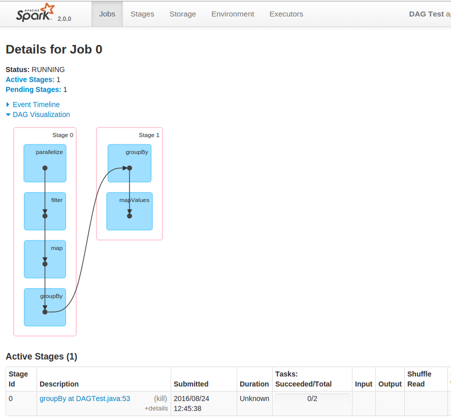
This graph was generated to following code:
List<String> animals = Arrays.asList("cat", "dog", "fish", "chicken");

JavaPairRDD> paired = CONTEXT.parallelize(animals)
  .filter(name ->  name.length() > 3)
  .map(name -> name.length())
  .groupBy(nameLength -> "The name has a length of " + nameLength);
paired.collect();
This post introduces the main concepts of background of Spark's jobs execution. The first part talks about the concept used to plan tasks - directed acyclic graph. It explains the characteristics of this type of graph. The second part brings this general information to Spark's environment. The 3rd part is the most precious because it presents what happens once DAG is defined by Spark. The last part shows how we analyze all activity related to DAG through programming API or web UI.
Data Engineering Design Patterns
Looking for a book that defines and solves most common data engineering problems? I wrote
one on that topic! You can read it online
on the O'Reilly platform,
or get a print copy on Amazon.
I also help solve your data engineering problems contact@waitingforcode.com 📩