
Previously we've learned about the vertices and edges representations in Apache Spark GraphX. At this moment to not introduce too many new concepts at once, we deliberately omitted the discovery of edges partitioning. Luckily, a new week comes and it lets us discuss that.
What would it take for you to trust your Databricks pipelines in production?
A 3-day bug hunt on a 3-person team costs up to €7,200 in lost engineering time. This workshop teaches you to prevent that — unit tests, data tests, and integration tests for PySpark and Databricks Lakeflow, including Spark Declarative Pipelines.

Konieczny
This post is divided into 4 sections. Each one describes one of the available edge partitioning strategies. It starts by 3 pretty simple and at the same time, pretty inefficient strategies. The last section talks about one strategy that outperforms all of them.
1 dimension edge partitioning
It's the simplest strategy that we meet very often in the data world. It uses the idea of the modulo division to figure out the number of the partition. The exact formula is (vertexId * 1125899906842597) % numPartitions. The result of that is the collocation of all edges with the same source vertex in the same partition. It's pretty dangerous because very often in the graph we have to deal with Power Law, i.e. the situation when some vertex has an order of magnitude more edges than the second vertex in the list and the second vertex has the same order of magnitude difference with the third and so forth. It makes the partitions unbalanced:
  behavior of "1 dimension edge partitioning"

  it should "create balanced partitions" in {
    val partitionedEdges = (1 to 100).map(sourceId => EdgePartition1D.getPartition(sourceId, 1, 2))

    val partitioningResult = partitionedEdges.groupBy(nr => nr).mapValues(edges => edges.size)

    partitioningResult should have size 2
    partitioningResult(0) shouldEqual 50
    partitioningResult(1) shouldEqual 50
  }

  it should "create unbalanced partitions" in {
    val partitionsNumber = 2
    // previous test had 1 edge for each of vertices. Here some of vertices have much more edges than the others
    val partitionedEdges = (1 to 100).flatMap(sourceId => {
      if (sourceId % 2 == 0) {
        (0 to 5).map(targetId => EdgePartition1D.getPartition(sourceId, targetId, partitionsNumber))
      } else {
        Seq(EdgePartition1D.getPartition(sourceId, 1, partitionsNumber))
      }
    })

    val partitioningResult = partitionedEdges.groupBy(nr => nr).mapValues(edges => edges.size)

    partitioningResult should have size 2
    partitioningResult(0) shouldEqual 300
    partitioningResult(1) shouldEqual 50
  }
Random vertex-cut partitioning
An improved version of the previous strategy is called random vertex-cut partitioning. It collocates the edges between the same vertices in the same partition: abs((sourceId, targetId).hashCode) % numPartitions. The formula shows clearly that the order of vertices matters, hence this partitioning strategy applies to the directions of edges. It results in a much better support for Power Law, except the case where some subset of vertices shares a lot of different types of edges together. It could be the case in bipartite graphs with customers and products. A customer could comment, buy, share and recommend his favorite product, creating so "hotspot" edges:
  it should "create almost balanced partitions" in {
    val partitionedEdges = (1 to 100).map(sourceId => RandomVertexCut.getPartition(sourceId, sourceId+200, 2))

    val partitioningResult = partitionedEdges.groupBy(nr => nr).mapValues(edges => edges.size)

    partitioningResult should have size 2
    partitioningResult(0) shouldEqual 42
    partitioningResult(1) shouldEqual 58
  }

  it should "create unbalanced partitions" in {
    val partitionsNumber = 3
    val partitionedEdges = (1 to 100).flatMap(sourceId => {
      if (sourceId % 2 == 0) {
        (0 to 10).map(_ => RandomVertexCut.getPartition(sourceId, 300+sourceId, partitionsNumber)) ++
          (0 to 10).map(_ => RandomVertexCut.getPartition(300+sourceId, sourceId, partitionsNumber))
      } else {
        Seq(RandomVertexCut.getPartition(sourceId, 200+sourceId, partitionsNumber))
      }
    })

    val partitioningResult = partitionedEdges.groupBy(nr => nr).mapValues(edges => edges.size)

    partitioningResult should have size 3
    partitioningResult(0) shouldEqual 430
    partitioningResult(1) shouldEqual 323
    partitioningResult(2) shouldEqual 397
  }
Canonical random vertex-cut partitioning
The 3rd strategy is similar to the previous one and we can notice that even by its name: canonical random vertex-cut partitioning. It also collocates the edges between the same vertices in the same partition. But unlike the previous strategy, this one ignores the direction of the edge:
if (src < dst) {
        math.abs((src, dst).hashCode()) % numParts
      } else {
        math.abs((dst, src).hashCode()) % numParts
      }
Therefore, the risk of unbalanced partitions for the vertices sharing more than 1 edge, independently on the direction, is smaller than for random vertex-cut strategy:
  it should "create almost balanced partitions" in {
    val partitionedEdges = (1 to 100).map(sourceId => CanonicalRandomVertexCut.getPartition(sourceId, sourceId+200, 2))

    val partitioningResult = partitionedEdges.groupBy(nr => nr).mapValues(edges => edges.size)

    partitioningResult should have size 2
    partitioningResult(0) shouldEqual 42
    partitioningResult(1) shouldEqual 58
  }

  it should "create more balanced partitions than random vertex-cut" in {
    val partitionsNumber = 3
    val partitionedEdges = (1 to 100).flatMap(sourceId => {
      if (sourceId % 2 == 0) {
        (0 to 10).map(_ => CanonicalRandomVertexCut.getPartition(sourceId, 300+sourceId, partitionsNumber)) ++
          (0 to 10).map(_ => CanonicalRandomVertexCut.getPartition(300+sourceId, sourceId, partitionsNumber))
      } else {
        Seq(CanonicalRandomVertexCut.getPartition(sourceId, 200+sourceId, partitionsNumber))
      }
    })

    val partitioningResult = partitionedEdges.groupBy(nr => nr).mapValues(edges => edges.size)

    partitioningResult should have size 3
    partitioningResult(0) shouldEqual 397 // vs 430 for random vertex-cut
    partitioningResult(1) shouldEqual 345 // vs 323 for random vertex-cut
    partitioningResult(2) shouldEqual 408 // vs 397 for random vertex-cut
  }
2 dimensions edge partitioning
The last and at the same time, the most advanced partitioning strategy is called 2 dimensions edge partitioning. At first glance we could think that it uses 2 vertices present in the edge for the partitioning, but it's not completely like that. The algorithm uses the following formulas to compute the partition number:
      if (numParts == ceilSqrtNumParts * ceilSqrtNumParts) {
        // Use old method for perfect squared to ensure we get same results
        val col: PartitionID = (math.abs(src * mixingPrime) % ceilSqrtNumParts).toInt
        val row: PartitionID = (math.abs(dst * mixingPrime) % ceilSqrtNumParts).toInt
        (col * ceilSqrtNumParts + row) % numParts

      } else {
        // Otherwise use new method
        val cols = ceilSqrtNumParts
        val rows = (numParts + cols - 1) / cols
        val lastColRows = numParts - rows * (cols - 1)
        val col = (math.abs(src * mixingPrime) % numParts / rows).toInt
        val row = (math.abs(dst * mixingPrime) % (if (col < cols - 1) rows else lastColRows)).toInt
        col * rows + row

      }
In both cases the algorithm uses source and destination vertices to compute the partition's number. The Scaladoc of this method uses the matrix to give an example of the distribution. Also the variable names, col and rows, automatically make thinking about this structure. We can consider then that the formula computes in fact the cell of the matrix where the given edge will be stored. The cell corresponds to the partition number. I tried to illustrate that on a simple example below:
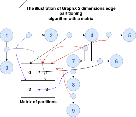
The first version of the above algorithm is used when the partitions number is a perfect square value (4, 9, 16, 25, ...). For the case of a not perfect square number of partitions, the strategy is similar. The difference is the last column that can have a different number of rows that the others.
Even though the algorithm works better when N is a perfect square, it doesn't mean that in the opposite case it performs poorly. We can see some very little differences in the following test case :
  it should "perform well for perfect square N" in {
    val partitionsNumber = 9
    val partitionedEdges = (1 to 100).flatMap(sourceId => {
      if (sourceId % 2 == 0) {
        (0 to 10).map(_ => EdgePartition2D.getPartition(sourceId, 300+sourceId, partitionsNumber))
      } else {
        Seq(EdgePartition2D.getPartition(sourceId, 200+sourceId, partitionsNumber))
      }
    })

    val partitioningResult = partitionedEdges.groupBy(nr => nr).mapValues(edges => edges.size)

    partitioningResult should have size 6
    partitioningResult(0) shouldEqual 176
    partitioningResult(2) shouldEqual 17
    partitioningResult(3) shouldEqual 17
    partitioningResult(4) shouldEqual 187
    partitioningResult(8) shouldEqual 187
  }

  it should "perform a little bit worse for not perfect square N" in {
    val partitionsNumber = 8
    val partitionedEdges = (1 to 100).flatMap(sourceId => {
      if (sourceId % 2 == 0) {
        (0 to 10).map(_ => EdgePartition2D.getPartition(sourceId, 300+sourceId, partitionsNumber))
      } else {
        Seq(EdgePartition2D.getPartition(sourceId, 200+sourceId, partitionsNumber))
      }
    })

    val partitioningResult = partitionedEdges.groupBy(nr => nr).mapValues(edges => edges.size)
    partitioningResult should have size partitionsNumber
    partitioningResult(0) shouldEqual 92
    partitioningResult(1) shouldEqual 92
    partitioningResult(2) shouldEqual 103
    partitioningResult(3) shouldEqual 53
    partitioningResult(4) shouldEqual 63
    partitioningResult(5) shouldEqual 52
    partitioningResult(6) shouldEqual 132
    partitioningResult(7) shouldEqual 13
  }
The 2 dimensions edge partitioning strategy also guarantees that one vertex is replicated in at most 2 * √N machines:
  it should "guarantee each vertex on only 2 partitions" in {
    val partitionsNumber = 4
    val partitionedEdges = (1 to 100).flatMap(sourceId => {
      if (sourceId % 2 == 0) {
        (0 to 10).flatMap(_ => {
          val destinationId = 300+sourceId
          val partition = EdgePartition2D.getPartition(sourceId, destinationId, partitionsNumber)
          Seq((sourceId, partition), (destinationId, partition))
        })
      } else {
        val destinationId = 200+sourceId
        val partition = EdgePartition2D.getPartition(sourceId, destinationId, partitionsNumber)
        Seq((sourceId, partition), (destinationId, partition))
      }
    })

    val verticesOnPartitions = partitionedEdges.groupBy(vertexWithPartition => vertexWithPartition._1)
      .mapValues(vertexWithPartitions => vertexWithPartitions.map(vertexIdPartitionId => vertexIdPartitionId._2).distinct.size)
    val verticesWith1Partition = verticesOnPartitions.filter(vertexIdPartitions => vertexIdPartitions._2 == 1).size
    val verticesWith2Partitions = verticesOnPartitions.filter(vertexIdPartitions => vertexIdPartitions._2 == 2).size
    verticesOnPartitions.size shouldEqual (verticesWith1Partition + verticesWith2Partitions)
  }
The guarantee about at most 2 * √N partitions containing a vertex is interesting from the shuffle point of view. As you already know, for triplets operation GraphX moves the vertices to the edge partitions. And since we've a relatively small number (compared to other strategies) of partitions with particular vertex, the network communication is smaller.
Moreover, according to the benchmarks done by Facebook or Zhuoyue Zhao et., 2 dimensions edge partitioning strategy is the most efficient strategy by far for graphs at scale processed with Apache Spark GraphX.
This post described edge partitioning strategies available in Apache Spark GraphX. As we could see, the framework provides different modulo-based strategies. Some of them use only the source vertex id and hence expose the risk of unbalanced partitions for graphs suffering of Power Law. The others use edge vertices to figure out the partition. Their results are much better but still don't guarantee good processing performances. Fortunately, the 2 dimensions edge partitioning strategy offers much better performance. Aside from pretty good data processing times, it also guarantees that each vertex will be stored in at most 2 * √N partitions, reducing by that the amount of shuffled data in the case of triplets operation.
Data Engineering Design Patterns

Looking for a book that defines and solves most common data engineering problems? I wrote
one on that topic! You can read it online
on the O'Reilly platform,
or get a print copy on Amazon.
I also help solve your data engineering problems contact@waitingforcode.com 📩
Read also about Edge partitioning strategies here:
- A comparison of state-of-the-art graph processing systems InferSpark: Statistical Inference at Scale
Related blog posts:
Partitioning #bigdata graphs is hard because of Power Law. #ApacheSpark #GraphX proposes 4 edge partitioning strategies that I described in today's post https://t.co/FtMGPDm4jf
— Bartosz Konieczny (@waitingforcode) January 3, 2019