Time series - general notes

Temporal data is a little bit particular. It can be generated very frequently, as for instance every 500 ms or less. It's then important to store it efficiently and to allow quick and flexible reads. It's also important to know the specificities of time-series as a popular case of temporal data.

Data Engineering Design Patterns

Looking for a book that defines and solves most common data engineering problems? I'm currently writing one on that topic and the first chapters are already available in 👉 Early Release on the O'Reilly platform

I also help solve your data engineering problems 👉 contact@waitingforcode.com 📩

This post is called "general notes" since it presents the common points of time series from the bird's eye view. The first section explains the general points about time series. The next one focuses on the data characteristics of the time series while the last one tries to explain the technical solutions helping to put them in place.

General information

Time series belongs to the family of the temporal data, i.e. the values somehow related to the time concept (either a point in time or an interval). The main ordering domain of this data category is unsurprisingly the time (e.g. event time).

The time series is the subset of the temporal data. It's represented as a sequence of data points happened over a time interval. The happen-moment can occur either at regular or irregular interval. This regularity has a big influence on the amount of registered data. The regular registering every 1 second will generate much more data than an irregular one saving for instance ATM transactions.

The registering regularity brings the first points describing time series - the granularity. It defines the scale of the stored data and thus determines the level of information we can gather through it. The information contained in time series is quite important. It lets pretty easily to observe the trends (e.g. website real-time audience) and correlate the measurements with potentially impacting events.

Among the operations we can made with the time series we can find a lot of common points with classical RDBMS querying, as:

• aggregations over a time, e.g. average of a metric over the last 3 hours
• slicing - the retrieval of the metrics happened between two points in time
• rescaling - the operations on the data of different granularity, e.g. the data is stored with seconds granularity and the operations are made on hours

Data characteristics

The time series data can be described by the following concepts:

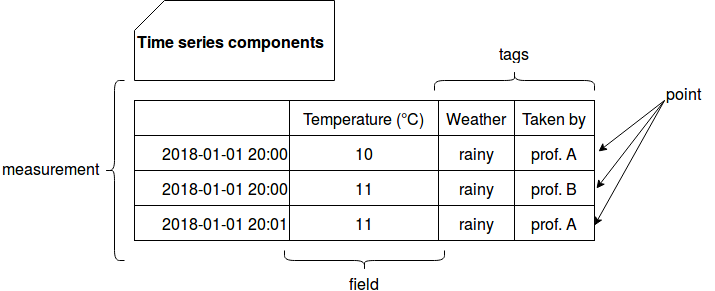
• measurement - it's the container for all below points. It's similar to a table from RDBMS world. As an example of the measurement we can consider the temperature measure taken every minute.
• point - represents a specific event occured at the register time.
• fields - this concept englobes all the values registered for the given point.
• tags - are the metadata associated with the registered measurements as a (key, value) pairs. Its main purpose consists on adding more context to the measure that can be later used to, for instance, slice the data or filter it. To our temperature measurement we can add a tags like: weather=(rainy or sunny or cloudy or windy ....).

To have a more precise context our temperature measurement example can look like in the table below:

The time series data character is also specific. It can be summarized by the following points:

• timestamped - since the measure is related to the time, it must be described by it. The timestamp acts like a primary key with the difference that it may not be unique. As you can see in the table above, 2 measures were taken for 20:00's temperature by different people. The time series are so a sequence of (timestamp, value) measurements ordered by timestamp.
• immutability - in-place changes happen rarely. But it doesn't mean that the data is not reprocessed. For example it can be reprocessed in order to create the aggregated metrics with smaller granularity for archiving purposes. The aggregates help to reduce the space taken by the initially registered values.
• unique - a measure must be identified uniquely. For instance we can't have 2 measures taken by the same person for given time period.
• time-sorted - usually the time series are a sorted sequence of points representing events occurred in time. Even though they can arrive in disorder, most of the time they're represented as ordered sequence of events.
• freshness - depending on the measurement regularity, the time series will often be fresh data. It means that the writes dominate the workload and are often done in near-real time (within seconds after the event time) and that rarely the old data is inserted.
• calendar - it's a pattern how often new observations are recorded.
• compaction - a part of data considered as old can be compacted. A compaction solution can be the aggregation quoted in the first point of this list. Here instead of storing minute-recorded points we create the aggregates for commonly used measurements, for instance every 10 minutes.
• bulk removal - it's somehow related to the previous point. Once the historical measures are aggregated we don't need to store them at fine grained level. Instead they can be removed. The most often the removal occurs for batches of data (e.g. all points between 2010-01-01 00:00 and 2010-02-01 00:00) and rarely for particular point.
• storage - depending on the underlying storage, the measurement can be stored as an array of points ([(2018-01-01 10:00, temperature: 10), (2018-01-01 10:01, temperature: 10)]) or as the arrays of timestamps and values ([2018-01-01 10:00, 2018-01-01 10:01], [10, 10]). As you can easily deduce, the former format is reserved to row-oriented store and the latter one for column-oriented.
• highly compressible - time-series data can be pretty well compressed. One of fitting compression algorithms can be the delta one that stores only the difference between the first and the latter points. So the entries [10, 11, 15, 9] will be stored as [10, 1, 5, -9]. It applies as well for values as for timestamps.
• read pattern - very often the data is generated as (timestamp, metric) pair but the reading path is done by metric, e.g. we want to know the temperature evolution during last 3 months. It can be solved in 2 different ways. The first one consists on adding an extra computation power for reading. The second one is the formatting the data before adding it to the database (format optimized for read patterns).

The architectures for time series

In "Comparison of Time Series Databases" Andreas Bader classifies the time series databases according to the criteria emphasizing the technologies behind the databases used to store time series. Among them we can distinguish 3 technical approaches:

• requirement on 3rd-part NoSQL - here the time series are backed by another storage. Often the storage is key-value data store as Cassandra (KairosDB) or HBase (OpenTSDB)
• RDBMS - the time series can sometimes be stored in the classical RDBMS. However this approach must be evaluated carefully because the relational databases scales horizontally very hard.
  An example of schema for our temperature measurement sample could be:
  

  CREATE TYPE weather_type AS ENUM ('rainy', 'cloudy', 'sunny', 'windy');
  
  
  CREATE TABLE weather_measurement (
    observation_time TIMESTAMP NOT NULL,
    observation_author VARCHAR(10) NOT NULL,
    temperature INT NULL,
    weather weather_type NOT NULL,
    PRIMARY KEY(observation_time, observation_author)
  );

• no requirement on any other database - the used storage is either proprietary or universal. One of examples for the second case is Druid platform based on Lambda architecture

The "Comparison of Time Series Databases" gives also some insight on the evaluation of the architecture well suited for time series data:

• Distribution and Clusterability - includes HA, scalability and load balancing. This group of requirements helps to ensure that the high volume of data will be still read efficiently and that the reading will be available even in the case of failure of some of nodes.
• Available functions - the database should make possible to query with aggregation functions (average, sum, count...) and also execute range queries as already told in the first section.
• Long-term storage - this feature determines how the TDBS is adapted for long-term storage . As already told, the granularity has an important impact on the volume of stored data. The storage mechanism should be able to remove the old data or to store its aggregated forms.
• Granularity - the storage should not constraint the possible data granularities. If the business needs fine-grained values, it should not be a problem for a database to handle it.
• Interfaces and extensibility - this point is related to the available APIs and customization (e.g. through UDF). It's quite important for all software decisions.

This post summarized the basic information about the time series. As we could see in the first part, they're a subset of temporal data, i.e. data sorted by the event time. This kind type of data is characterized by regular or irregular generation. The database storing time series must be resilient and easily scalable since the volume of time series can grow very quickly. Moreover, it should support the requirement for long-term storage by supporting data removal and aggregation. As shown in the last section, different approaches exist to deal with that. The first ones are based on 3rd part NoSQL storages as Cassandra or HBase. The other ones use the classical RDBMS while the last category doesn't require any specific storage.