
By the end of 2018 I published a post about code generation in Apache Spark SQL where I answered the questions about who, when, how and what. But I omitted the "why" and cozos created an issue on my Github to complete the article. Something I will try to do here.
What would it take for you to trust your Databricks pipelines in production?
A 3-day bug hunt on a 3-person team costs up to €7,200 in lost engineering time. This workshop teaches you to prevent that — unit tests, data tests, and integration tests for PySpark and Databricks Lakeflow, including Spark Declarative Pipelines.

Konieczny
In this post I will deep delve into "Apache Spark as a Compiler: Joining a Billion Rows per Second on a Laptop" post and focus on the points listed as the drawbacks of the previous execution model (Volcano).
Wholestage vs no wholestage
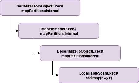
When the whole stage code generation is disabled, Apache Spark will use physical plans doExecute() method. As stated in the whole stage code generation documentation, such execution works by first calling the doExecute on the child node and applying the transformation logic on the results generated by this node. Below you can find a more illustrative example of what happens when whole stage code generation is disabled for that code:
val sparkSession: SparkSession = SparkSession.builder().appName("Spark SQL codegen test")
  .master("local[*]")
  .config("spark.sql.codegen.wholeStage", "false")
  .getOrCreate()
import sparkSession.implicits._
val dataset = Seq(("A", 1, 1), ("B", 2, 1), ("C", 3, 1), ("D", 4, 1), ("E", 5, 1)).toDF("letter", "nr", "a_flag")

dataset.filter("letter != 'A'")
  .map(row => row.getAs[String]("letter")).count()
The same query executed with whole stage generation enabled looks like:
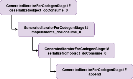
Although the execution is quite similar since the framework calls a doConsume of every physical node, in reality it's different. And the difference comes from the generated code which concatenates all operations in a single code unit (methods body omitted for clarity):
// ...
/* 006 */ final class GeneratedIteratorForCodegenStage1 extends org.apache.spark.sql.execution.BufferedRowIterator {
// ...
/* 019 */
/* 020 */   public void init(int index, scala.collection.Iterator[] inputs) {
/* 021 */     partitionIndex = index;
// ...
/* 031 */   }
/* 032 */
/* 033 */   private void mapelements_doConsume_0(org.apache.spark.sql.Row mapelements_expr_0_0, boolean mapelements_exprIsNull_0_0) throws java.io.IOException {
// ...
/* 058 */     serializefromobject_doConsume_0(mapelements_value_1, mapelements_isNull_1);
/* 060 */   }
/* 061 */
/* 062 */   private void deserializetoobject_doConsume_0(InternalRow inputadapter_row_0, UTF8String deserializetoobject_expr_0_0, boolean deserializetoobject_exprIsNull_0_0, int deserializetoobject_expr_1_0, int deserializetoobject_expr_2_0) throws java.io.IOException {
// ...
/* 096 */     mapelements_doConsume_0(deserializetoobject_value_0, false);
/* 098 */   }
/* 099 */
/* 100 */   private void serializefromobject_doConsume_0(java.lang.String serializefromobject_expr_0_0, boolean serializefromobject_exprIsNull_0_0) throws java.io.IOException {
// ...
/* 122 */     append((deserializetoobject_mutableStateArray_0[4].getRow()));
/* 124 */   }
/* 125 */
/* 126 */   protected void processNext() throws java.io.IOException {
/* 127 */     while (inputadapter_input_0.hasNext() && !stopEarly()) {
// ..
/* 135 */       deserializetoobject_doConsume_0(inputadapter_row_0, inputadapter_value_0, inputadapter_isNull_0, inputadapter_value_1, inputadapter_value_2);
/* 136 */       if (shouldStop()) return;
/* 137 */     }
/* 138 */   }
/* 139 */
/* 140 */ }
And despite these differences, the physical plans remain almost the same (* - whole stage code generation mark):
# no whole stage code gen == Physical Plan == SerializeFromObject [staticinvoke(class org.apache.spark.unsafe.types.UTF8String, StringType, fromString, input[0, java.lang.String, true], true, false) AS value#16] +- MapElements, obj#15: java.lang.String +- DeserializeToObject createexternalrow(letter#7.toString, nr#8, a_flag#9, StructField(letter,StringType,true), StructField(nr,IntegerType,false), StructField(a_flag,IntegerType,false)), obj#14: org.apache.spark.sql.Row +- LocalTableScan [letter#7, nr#8, a_flag#9] # with whole stage code gen == Physical Plan == *(1) SerializeFromObject [staticinvoke(class org.apache.spark.unsafe.types.UTF8String, StringType, fromString, input[0, java.lang.String, true], true, false) AS value#16] +- *(1) MapElements , obj#15: java.lang.String +- *(1) DeserializeToObject createexternalrow(letter#7.toString, nr#8, a_flag#9, StructField(letter,StringType,true), StructField(nr,IntegerType,false), StructField(a_flag,IntegerType,false)), obj#14: org.apache.spark.sql.Row +- LocalTableScan [letter#7, nr#8, a_flag#9]
Pre-codegen - Volcano model
The "no-whole-code-generation" execution uses a model called Volcano Model (aka Iterator Model). There are many great articles explaining it in detail so here I will only recall the simplified version. Every operation in this model is composed of 3 methods:
- open() - initializes a state
- next() - produced an output
- close() - cleans up the state
Knowing that, we can simply translate an Apache Spark code composed of filter and select operations like:
scan iterator -- next() --> select iterator -- next() --> filter iterator -- next() --> output iterator
As you can see, the idea is to get the data by calling child next() method every time. This abstraction was quite popular because of its simplicity. Every step in the pipeline is defined exactly with the same interface. At the same time, this advantage was also a drawback since the compiler doesn't know exactly what .next() it has to call. And that's the first drawback described in the original Databricks post about the new execution model (quotes below).
Virtual functions
No virtual function dispatches: In the Volcano model, to process a tuple would require calling the next() function at least once. These function calls are implemented by the compiler as virtual function dispatches (via vtable). The hand-written code, on the other hand, does not have a single function call. Although virtual function dispatching has been an area of focused optimization in modern computer architecture, it still costs multiple CPU instructions and can be quite slow, especially when dispatching billions of times.
In that description I see 2 important points to clarify, virtual functions and virtual function dispatches. In simple terms, virtual functions are like Java's abstract methods. They're declared but they are implemented only in the sub-classes, so when you're doing:
public abstract class A {
  public abstract xx();
}

public class B extends A {
   override public xx() {}
}
public class C extends A {
   override public xx() {}
}

A b = new B();
b.xx();
The compiler doesn't know (simplified vision) what implementation of A should be called. And to figure it out, it has to look at vtable. A vtable is a structure with all virtual function entries. For every entry it stores a pointer to the definition of this function (C++ example):
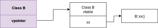
The virtual function dispatch uses the vpointer under each class, goes to the corresponding virtual table and only at the end it resolves the code to execute. In the case of the whole code generated stage, since everything happens inside 1 class where the implementations are clearly defined, the virtual functions don't exist.
Memory vs CPU registers
Intermediate data in memory vs CPU registers: In the Volcano model, each time an operator passes a tuple to another operator, it requires putting the tuple in memory (function call stack). In the hand-written version, by contrast, the compiler (JVM JIT in this case) actually places the intermediate data in CPU registers. Again, the number of cycles it takes the CPU to access data in memory is orders of magnitude larger than in registers.
To understand this part, let me introduce the parts of computer architecture with corresponding latencies (only for illustration purpose, the measures are for 2012 so they certainly changed but I didn't find an updated example):
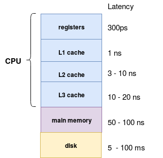
When I saw this picture, I met for the first time the ps unit. A ns stands for nanosecond which is one billionth of one second (1 / 1 000 000 00). The ps represents a picosecond and it's one trillionth of one second (1 / 1 000 000 000 000). As stated in the introduction quote, in Volcano Model data is very far from the registers and its access time increases significantly.
Loop unrolling
Loop unrolling and SIMD: Modern compilers and CPUs are incredibly efficient when compiling and executing simple for loops. Compilers can often unroll simple loops automatically, and even generate SIMD instructions to process multiple tuples per CPU instruction. CPUs include features such as pipelining, prefetching, and instruction reordering that make executing simple loops efficient. These compilers and CPUs, however, are not great with optimizing complex function call graphs, which the Volcano model relies on.
A loop unrolling feature belongs to time - space trade-offs family because it trades decreased execution time in for increased function size. It means that a for loop like this one:
for (i = 0; i < 100; i++):
   do_something(i)
can be rewritten by the compiler to this optimized (loop unrolled) form:
for (i = 0; i < 100; i += 2):
   do_something(i)
   do_something(i+1)
The unrolled version will execute only a half of the operations of the not unrolled loop and potentially will also represent a gain in terms of hardware management (jumps, conditional branches). Good news, loop unrolling doesn't apply only to the for loops. It also works on while:
# normal
while (condition):
   do_something()

# unrolled
while (condition):
  do_something()
  if (!condition): break
  do_something()
  if (!condition): break
  do_something()
Since whole stage code is an iterator processing every new row in a while loop, it's a subject for an eventual loop unrolling optimization. Optimizing Volcano Model is much harder than that.
In this post I tried to popularize the "why" of code generation in Apache Spark SQL. I didn't invent new reasons though. Instead, I only clarified the ones listed in the Databricks blog post introducing code generation feature ("Apache Spark as a Compiler: Joining a Billion Rows per Second on a Laptop"). Maybe one day I'll have enough time to delve into the topic of compiled queries and therefore, will complete the 3 points of this article. Meantime, I hope this popularized version will help to understand the "why".
Data Engineering Design Patterns

Looking for a book that defines and solves most common data engineering problems? I wrote
one on that topic! You can read it online
on the O'Reilly platform,
or get a print copy on Amazon.
I also help solve your data engineering problems contact@waitingforcode.com 📩
Read also about The why of code generation in Apache Spark SQL here:
- SPARK-12795 Whole stage codegen Apache Spark as a Compiler: Joining a Billion Rows per Second on a Laptop Spark SQL Codegen: Why Vectorized and Compiled Queries — Part 1 A Deep Dive into Query Execution Engine of Spark SQL Understanding Virtual Tables in C++ Advanced databases Loop unrolling JVM JIT - Loop Unrolling
Related blog posts:
- Introduction to custom optimization in Apache Spark SQL
- The who, when, how and what of Apache Spark SQL code generation
- Apache Spark and off-heap memory
- Multiple SparkSession for one SparkContext
- Apache Spark SQL, Hive and insertInto command
A reader asked on my Github to complete my previous post about code generation with the "why" part. To do that, I illustrated the 3 initial reasons presented in "Apache Spark as a Compiler: Joining a Billion Rows per Second on a Laptop" https://t.co/mOMXqF7473
— Bartosz Konieczny (@waitingforcode) September 28, 2019