
When you start a Structured Streaming job, your Spark UI will get a new tab in the menu where you follow the progress of the running jobs. In the beginning this part may appear a bit complex but there are some visual detection patterns that can help you understand what's going on.
What would it take for you to trust your Databricks pipelines in production?
A 3-day bug hunt on a 3-person team costs up to €7,200 in lost engineering time. This workshop teaches you to prevent that — unit tests, data tests, and integration tests for PySpark and Databricks Lakeflow, including Spark Declarative Pipelines.

Konieczny
In this blog post you're going to discover some visual patterns that - hopefully - will help you spot the issues with your job more easily.
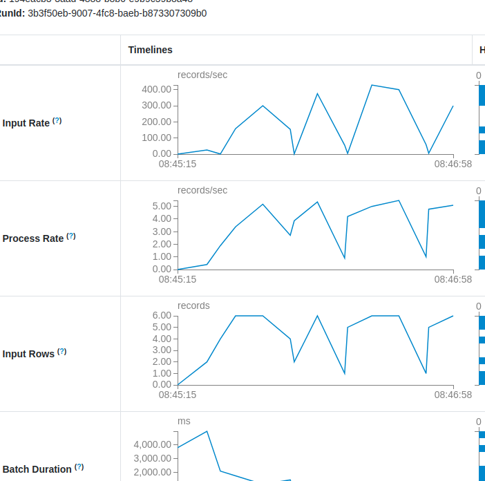
Input rate and process rate
The first situation you certainly want to avoid is to see your input rate higher than the processing rate. Both measures are displayed per second and are calculated by ProgressReporter#finishTrigger as follows:
protected def finishTrigger(hasNewData: Boolean, hasExecuted: Boolean): Unit = {
  // ...
  val sourceProgress = sources.distinct.map { source =>
    val numRecords = executionStats.inputRows.getOrElse(source, 0L)
  // ...
  val processingTimeMills = currentTriggerEndTimestamp - currentTriggerStartTimestamp
  val processingTimeSec = Math.max(1L, processingTimeMills).toDouble / MILLIS_PER_SECOND

  val inputTimeSec = if (lastTriggerStartTimestamp >= 0) {
     (currentTriggerStartTimestamp - lastTriggerStartTimestamp).toDouble / MILLIS_PER_SECOND
  } else {
    Double.PositiveInfinity
  }


  inputRowsPerSecond = numRecords / inputTimeSec,
  processedRowsPerSecond = numRecords / processingTimeSec,
From the previous snippet you can see that:
- Process rate is based on the current micro-batch. For example, for a micro-batch that lasted for 1 minute and processed 100 records, the rate will be calculated as 100 / 60, so it will be of 1.6 records per second.
- Input rate is based on the current and previous micro-batches. For example, if the previous run started at 10:00 and the current run started at 10:01, and the current micro-batch processed 100 records, the input rate will be calculated as 100 / 60, so it'll be 1.6 records per second.
Unfortunately, the perfect rate is rarely the case and very often you'll observe some differences. To understand it better, let's take a visual example this time. In the next schema you can see a timeline with the micro-batches configured at a regular processing time trigger interval of 20 seconds. As you can notice, the micro-batches don't respect the trigger because of some unexpected processing issues. The difference between the second and the third runs is 40 seconds:
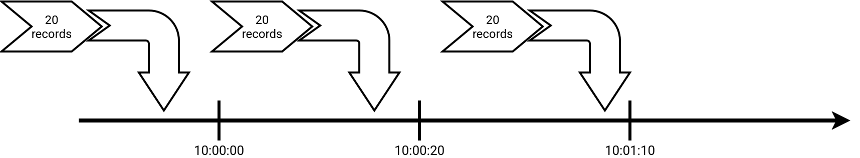
Consequently, the third micro-batch will have the input rate of 1 (20 input rows divided by 20 seconds interval between the beginning of the previous and the current micro-batch), but its process rate will be only 0.5 (20 input rows divided by 40 seconds micro-batch duration). In other words, the job takes more data that it can process with the actual compute power. To mitigate this issue you can then add new resources that should increase the processing parallelism and therefore, increase the process rate (the micro-batch will be faster, then the process rate will be higher).
Small process rate is often related to too big Batch duration. As you can see in the next picture, the batch duration is continuously increasing which leads to the process rate lower than the input rate:
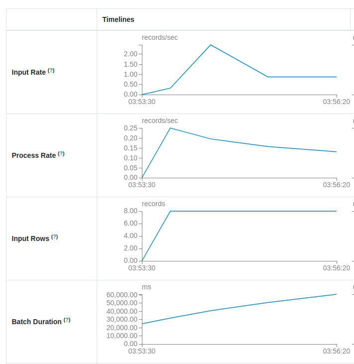
You saw it in the code before, both rates are highly dependent on the batch duration. Whenever the duration increases, the process rate and input rate decreases. However, as they operate at different micro-batches - the current micro-batch for the process rate and the previous with the current for the input rate - their values won't degrade at the same time. Let's analyze a hypothetical scenario where:
- Stable increased batch duration represents a micro-batch with the duration increased from 20 to 40 seconds
- Increasing batch duration represents a micro-batch with a continuously increasing duration
- Decreasing batch duration represents a micro-batch that after a sudden duration increase, got some better results.
| scenario | micro-batch | processing time (sec) | process rate / sec | input rate / sec |
|---|---|---|---|---|
| stable increased batch duration | 1 | 20 | 1 | 0 |
| stable increased batch duration | 2 | 20 | 1 | 1 |
| stable increased batch duration | 3 | 40 | 0.5 | 1 |
| stable increased batch duration | 4 | 40 | 0.5 | 0.5 |
| stable increased batch duration | 5 | 40 | 0.5 | 0.5 |
| increasing batch duration | 1 | 20 | 1 | 0 |
| increasing batch duration | 2 | 20 | 1 | 1 |
| increasing batch duration | 3 | 40 | 0.5 | 1 |
| increasing batch duration | 4 | 50 | 0.4 | 0.5 |
| increasing batch duration | 5 | 60 | 0.33 | 0.4 |
| increasing batch duration | 6 | 70 | 0.28 | 0.33 |
| increasing batch duration | 7 | 80 | 0.25 | 0.28 |
| decreasing batch duration | 1 | 20 | 1 | 0 |
| decreasing batch duration | 2 | 20 | 1 | 1 |
| decreasing batch duration | 3 | 40 | 0.5 | 1 |
| decreasing batch duration | 4 | 30 | 0.66 | 0.5 |
| decreasing batch duration | 5 | 25 | 0.8 | 0.66 |
| decreasing batch duration | 6 | 20 | 1 | 0.8 |
Metadata verdant
After this pretty long section, let's see another graph that can put you into trouble, the Operation duration. It represents more detailed information on how each micro-batch performed. The details are limited to the actions made by each micro-batch which are: metadata fetching, query planning, data processing, and checkpointing. In a healthy scenario, the dominant color should be orange. You should see the operation duration graph similar to:
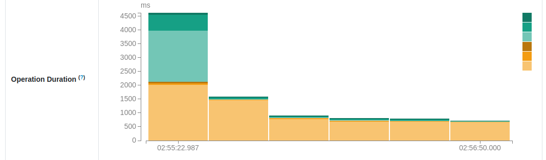
💡 Anormal-normal first micro-batch
The first micro-batch is special as it's often the first communication between your job and your data source(s). The job needs to do more work and for example in Apache Kafka, the job will need to list the available partitions, get the offsets, build the offsets ranges to process... All this makes the first micro-batch spending more time on the metadata than the others.
However, sometimes you may see this graph changing the dominant color to green, like here:
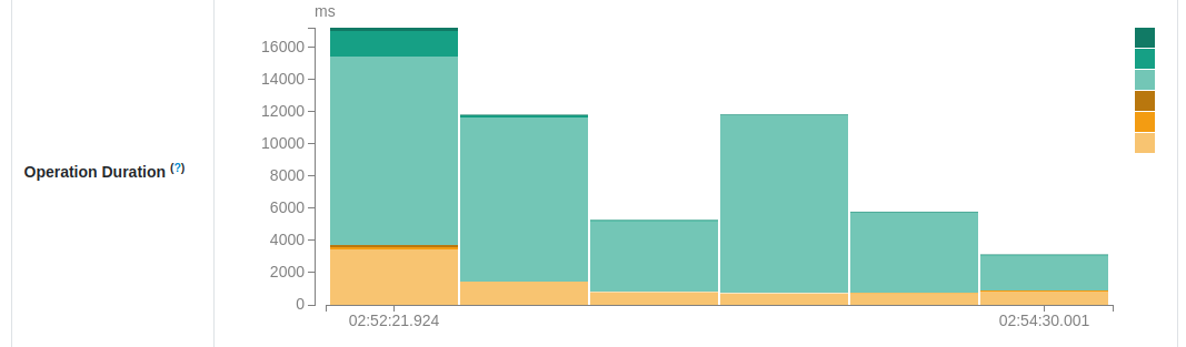
You should read this change as: my processing logic is probably fine but the communication between my job and the data source(s) or the checkpoint location is in trouble. In other words, your job might be spending more time on preparing the data for processing rather than on processing itself.
One of the greatest examples of this issues is file data source on the cloud object stores that runs a listing operation. If your input location never gets cleaned, your Structured Streaming job will have more and more files (objects) to list. Obviously, the operation that took 100 ms on 1000 files will now take 200 ms on 2000 files, ... 1 second on 10 000 files, ... the time only increases.
💡 Not only new objects
Although it sounds surprising, you might encounter listing latency issues for the object stores with the enabled versioning but without any lifecycle policy. I encountered one issue in the past and disabling the versioning - as it was blindly enabled to follow some abstract guidelines - greatly reduced the listing time of the Structured Streaming job. You'll find some details why in I'm experiencing performance degradation after enabling bucket versioning.
To mitigate this issue you need to address the data source problems. For the objects listing it can be streaming created files from a message queue upon configuring the delivery on your cloud provider (e.g. S3 notifications delivered on SQS), or using Databricks Auto Loader.
Hiking
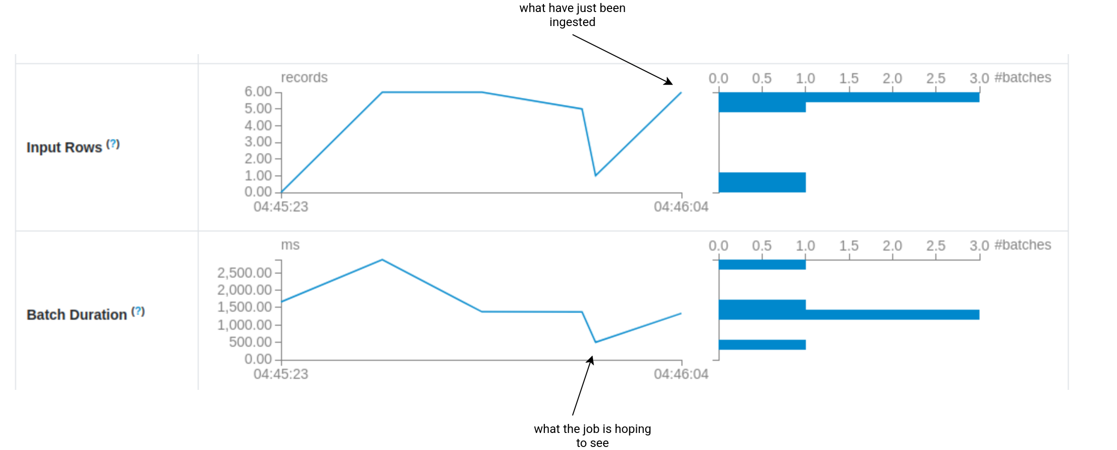
Another alarming pattern you can observe in Spark UI looks like hiking. Just take a look:
As you can see the job is facing some irregularities. There are times where our streaming application has a lot of work to do and other periods where there is almost no data to process. The reasons for that can be twofold. The issue is either on the data producer's side, or on your side (simple as it).
If your data producer generates data irregularly and you run your streaming job continuously (= aka process data as soon as possible), there might be periods when the job runs on the producer's smaller input. To mitigate this you can try to configure a processing time trigger and try to optimize the resources usage by - ideally - always processing the same data volume.
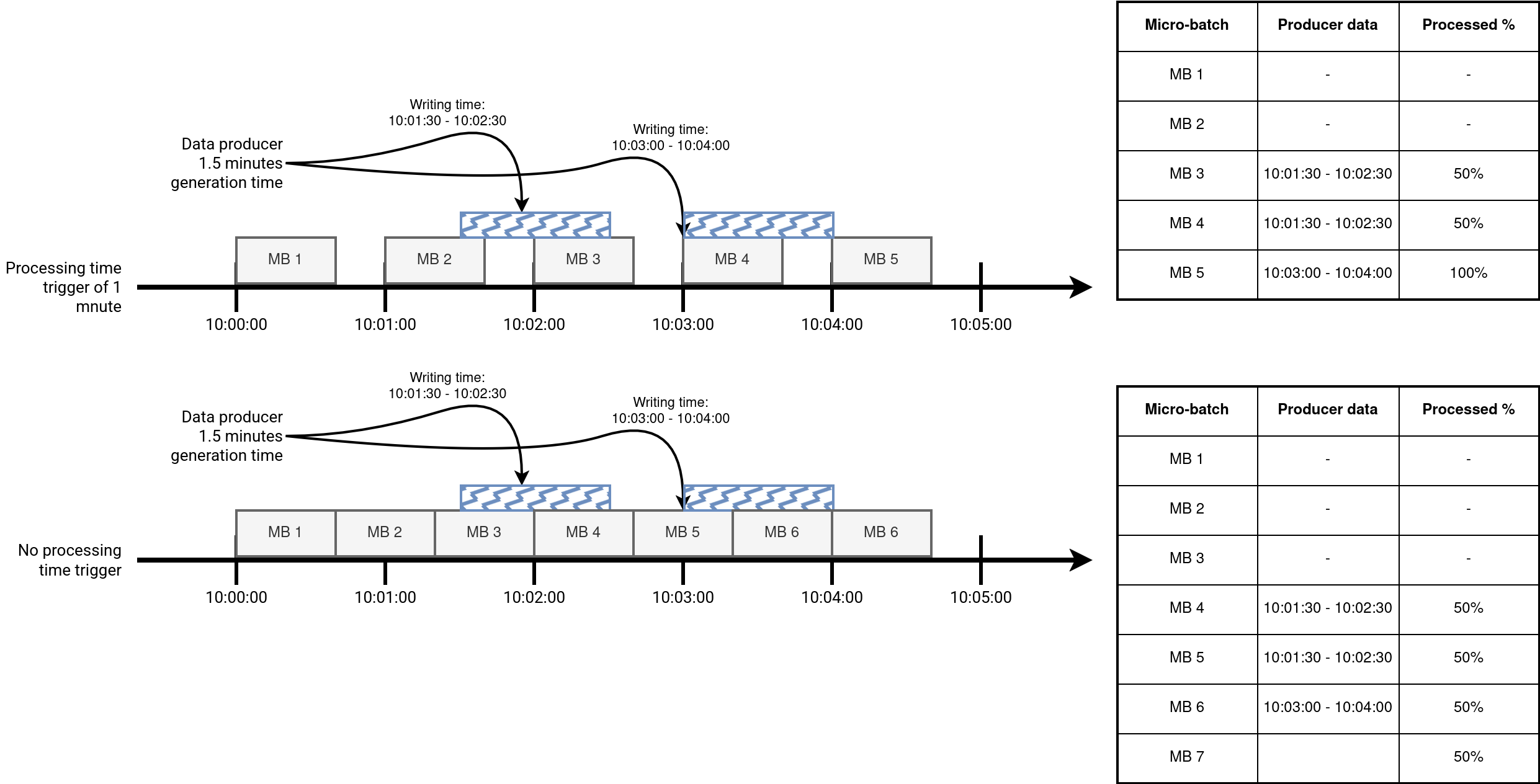
But there can be an opposite effect. If you run the job at a processing time interval, let's say 1 minute, and your data producer generates data less regularly, like during one minute every 1.5 minutes, you might consider removing the processing time trigger to try running the job on smaller chunks of data more regularly, shown in the next schema:
If the problem is on your side, with each hike you'll probably notice an increased Batch duration. It means that the job is trying to keep the pace and when it thinks to make up its delay, new data has been added for processing. A good solution here would be to control the batch duration by adding more compute resources.
Slide
Besides hiking, the Spark UI of your Structured Streaming job can also show some slides. If you visit playgrounds with your kids - that's my case at the moment 😅 - that's the representation you will draw when you see things like this:
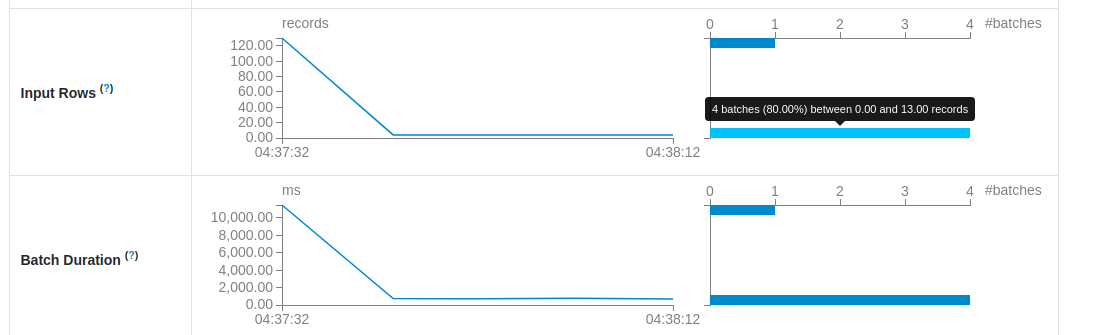
As you can see, the first micro-batch takes the most load. It happens when you start the job for the first time without any throughput controls. Let's imagine an Apache Kafka topic with a 7-days retention and a Structured Streaming job taking the whole load in the first run. If you have some luck, the first execution will succeed but will be slow. If you are less lucky, the first execution will simply fail and you will have to think about workarounds.
The easiest solution is to simply take the most recent data. If it's your case, the job will process all new data created after the start. However, historical data can be also useful in different scenarios, such as generating a consistent state for stateful jobs. In that case two choices might be:
- Set the throughput limitation and run the job with the expected trigger for the production real-time workload (e.g. processing time of 30 seconds). The job will take some time before it starts processing the real-time data but it will not need huge compute resources for that. If your production job doesn't expect throughput limits, you can stop the backfilling run, disable the throughput, and restart the job in the real-time mode.
- Use the AvailableNow trigger without the throughput limitation to process all data available prior to starting your job with the Structured Streaming API. After completing the run, you can start the job in normal real-time mode.
The sliding can also happen when your data producer suddenly generates much more data than usual. For example, the producer might encounter some issues, buffer the data to write, and flush the buffer only after one hour, leading to a lot of data to process on your side.
💡 Throughput limits
As you can see, due to the micro-batch nature, specifying the throughput limits can help keep your execution time and resources usage under control.
Stateful hiking
Finally, you can also notice some of the already described visual patterns in the stateful section. One of the most alarming one is the continuously increasing numbers of updates, as in the next screenshot where the state store doesn't stop from getting new entries:
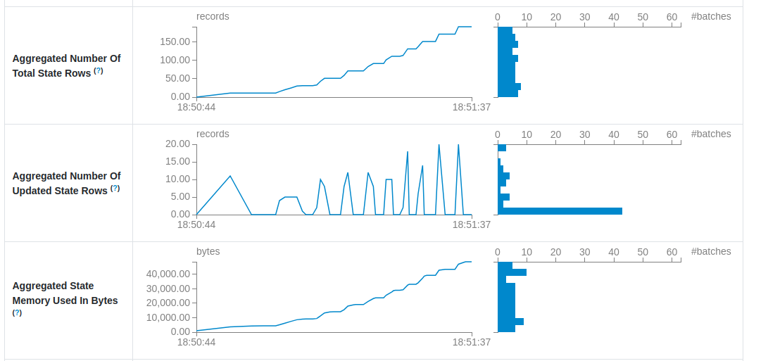
The issue may lead to a significant memory overhead with increased latency for checkpointing operation, and sometimes even to the job failures because of the allocated memory reached. Unfortunately, there is no single root cause. Among possible reasons you can find a wrong grouping key for the state rows which might create a new state for every input record, or yet too big watermark value leading to many updates and overall state increase.
If I had to summarize the observations from the blog post, I would say that any kind of deviation is not good. If your graph looks like a rollercoaster, your job will behave alike. There will be exciting moments but also the ones where you will be struggling to stabilize things. It's definitely better to keep things stable and under control, but unfortunately it's very hard to do!
Data Engineering Design Patterns

Looking for a book that defines and solves most common data engineering problems? I wrote
one on that topic! You can read it online
on the O'Reilly platform,
or get a print copy on Amazon.
I also help solve your data engineering problems contact@waitingforcode.com 📩
Read also about Apache Spark Structured Streaming UI patterns here:
Related blog posts:
- Spark Declarative Pipelines internals
- Spark Declarative Pipelines, going further
- Spark Declarative Pipelines 101