
I wish I could say once day: "I optimized Apache Spark pipelines in all possible ways". But I'm aware of the realty and that can be very hard to achieve. That's why I decided to rely on the experience shared by experienced Spark users in Spark+AI and, recently, Data+AI Summit, and write a summary list of interesting optimization tips from the past talks.
What would it take for you to trust your Databricks pipelines in production?
A 3-day bug hunt on a 3-person team costs up to €7,200 in lost engineering time. This workshop teaches you to prevent that — unit tests, data tests, and integration tests for PySpark and Databricks Lakeflow, including Spark Declarative Pipelines.

Konieczny
The article is organized into 5 sections, respectively about: partitions, code, skews, Garbage Collectors, and clusters. In the post, I focused only on the "hard" tips, without involving the recent optimizations brought by the Adaptive Query Execution engine. IMO, knowing all of them without the adaptive magic helps to understand better what happens when Apache Spark processes the data, and that's why I didn't include the AQE aspect here.
As you know, I didn't reinvent the wheel and based this blog post in various interesting past Spark+AI and Data+AI Summit talks. Credits for the tips go to:
- Daniel Tomes who gave one of the most complete optimizations tips talk I ever saw - Apache Spark Core - Practical Optimization
- Suganthi Dewakar who shared how to solve data skew at scale - Skew Mitigation For Facebook PetabyteScale Joins
- Rose Toomey who shared some key advices for Garbage Collection - Apache Spark At Scale in the Cloud
- Blake Becerra, Kaushik Tadikonda and Kira Lindke who shared their tips on, respectively, salting, GC and cluster configuration dependencies - Fine Tuning and Enhancing Performance of Apache Spark Jobs
- Yeshwanth Vijayakumar who spotted some differences of per-element and per-elements operations - How Adobe Does 2 Million Records Per Second Using Apache Spark!
- Jean-Yves Stephan and Julien Dumazert who shared the baseline parameters for Apache Spark jobs - How to Automate Performance Tuning for Apache Spark
Thank you all for the great talks!
Sizing partitions
Let's start with the partitions and some equations shared by Daniel Tomes. One of the most important partition points shared by Daniel in his talk was that the default value for spark.sql.shuffle.partitions. The default 200 is wrong. Or at least, it's wrong as long as you process more than 20GB of data. How to solve it? A few recommendations to keep in mind:
- shuffle partition should be between 100 and 200MB
- the number of shuffle partitions should be equal to stage input data size/target shuffle partition size
- try to optimize the resources use, if the number of partitions is lower than the number of available cores, set the number to partitions to be equal to the number of cores; to illustrate that, Daniel shared an interesting equation in this slide:
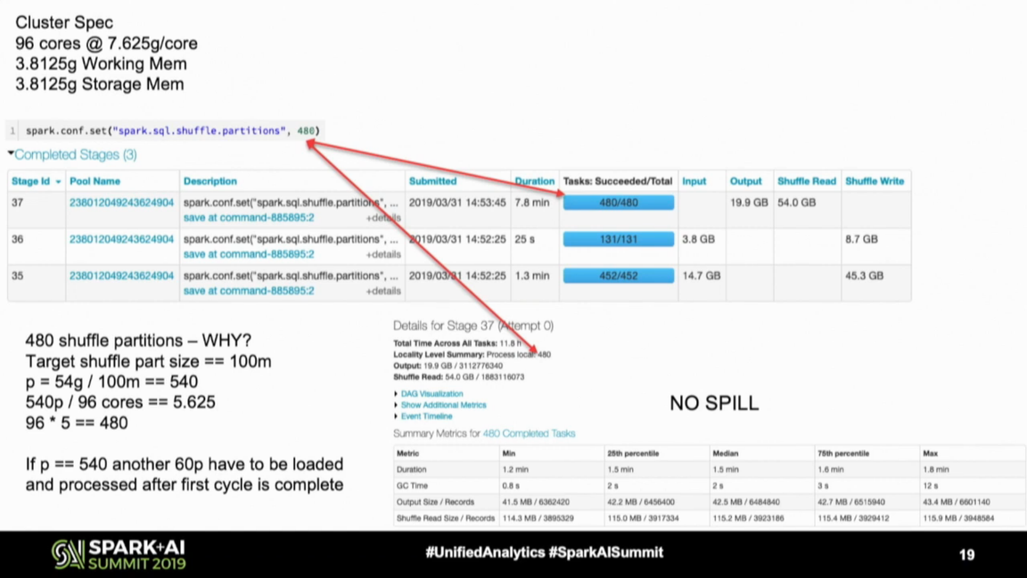 As you can see, the number of shuffle partitions is 480, not 540. Why? With the initial equation, approximately 35% of cores will remain idle in the last processed series of tasks (6 - 5.625). To optimize the resources use, Daniel rounded this number to 5 so that the compute power can be optimized (96 cores * 5 parallelism = 480 shuffle partitions).
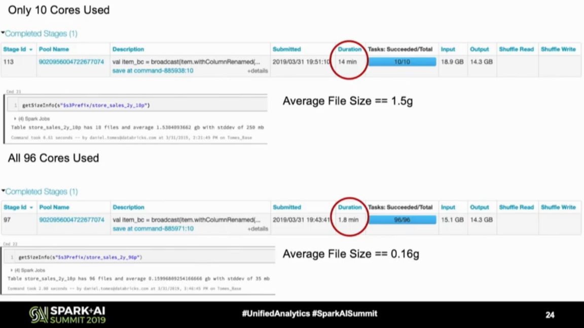
Bad shuffle partitions size can increase spills to the disk and also under optimize resources used on the cluster. But shuffle partitions is not the single number to optimize. The second one is about input partitions, and more exactly the spark.sql.files.maxPartitionBytes property. Daniel recommends to leave the default (128MB) unless:
- you want to increase the parallelism - especially if your cluster has more cores than dataset size/spark.sql.files.maxPartitionBytes; for example a cluster of 200 cores for a 200MB dataset will be inefficient with the default since only 2 partitions will be created (= 2 cores used).
- your input has a lot of or big nested fields or repetitive data - it can take much more place than expected
- you generate the data - if you perform some explode; i.e. 1 entry/attribute of your dataset generates 1 or more, then it's better to lower the input partition size to keep some room left for this extra data
- you use non vectorized UDFs because they can't be as efficiently serialized as the native functions
And finally, the output partitions - even though technically they don't exist the same way as the shuffle and input ones. Be aware that whenever you downscale the number of partitions before writing to the sink, the cores in your cluster will stay idle, and probably the writing will take longer, as shown below by Daniel:
The solution if you want to optimize writes and also keep files size consistent/bigger? You can create a smaller cluster to perform the compaction job or call OPTIMIZE if you use Databricks, as the next step in the ETL pipeline.
Coding tips
Shuffle multiplied
For the coding tips, let's start with the obvious one but apparently, not always respected:
inputDataset.repartition(10).groupByKey(user => user.id)
Obviously, we don't need to repartition the input data here since it will be "repartitioned" by the grouping operation. And since moving data is costly, eliminating such obvious duplicates can save some processing time.
Unpersist
Another tip shared by Daniel is about caching (persisting) a DataFrame. Doing that can have a beneficial effect on the processing time. But it can also have some negative impact if you cache a lot and "forget" to call unpersist() when the cache is not needed anymore.
Imagine that you persited the first DataFrame with memory+disk level, and it completely fitted to the main memory. However, you never unpersisted it and needed to persist another DataFrame in your application. This time, since the cache memory is already fully used, the caching will happen on disk and obviously will have a negative impact (= worse impact as it would be cached in memory).
NOT EXISTS instead of NOT IN
That's my favorite tip from the watched videos, using NOT EXISTS instead of NOT IN. In the query shown below you can see that the difference in time execution is huge!
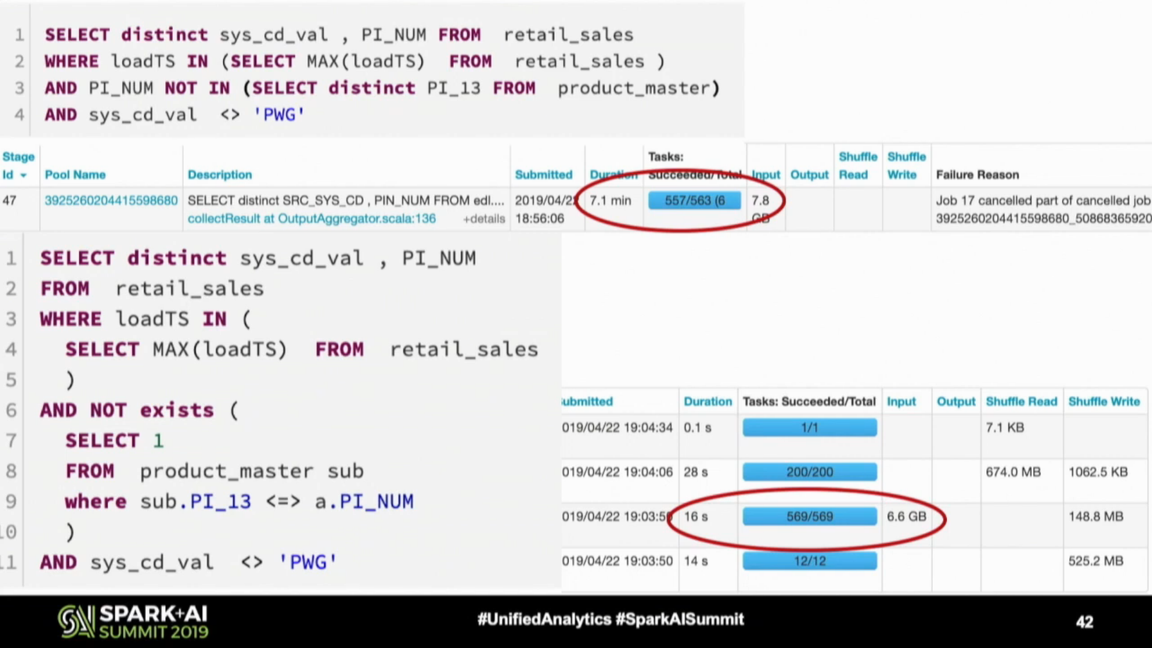
The NOT IN predicate is not the only reason for this improvement. Another one is the null safe equality preventing the inefficient Cartesian product calculation between nulls on both sides. I already added this NOT IN vs NOT EXISTS topic to my blogging backlog and hope to share more details with you soon!
SPARK-32290
Leanken Lin implemented an optimization for NOT IN execution in Apache Spark 3.1.1. Starting from this version, if the subquery uses a single column, the execution plan won't translate to the slow nested loop join. In consequence, the execution time for a query mentioned in SPARK-32290 decreased from 18 minutes to 30 seconds after this change! It can be your case too, if you use at least Apache Spark 3.1.1, and so without switching from NOT IN to NOT EXISTS.
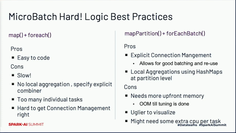
Batching
The next coding tips come from Yeshwanth Vijayakumar's talk about processing 2 millions of records per second with Apache Spark. According to Yeshwanth's experience, the map and foreach operations are often slower than mapPartitions and foreachBatch. So if you have a slow map operation, especially when you need some local aggregations or managing an external connection, maybe it's worth trying to rewrite it to mapPartitions and make a test? Be only aware that it may require some more compute or memory:
Handling skew
Aggregations
Data skews are another data processing challenge. Fortunately, there are some strategies to deal with them. The first and IMO the easiest strategy is to filter-out the unnecessary data as soon as possible; i.e. don't wait for the aggregated results to filter if you can do it before. But if it's not possible, Daniel Tomes shared a tip using random salting that should help to evenly distribute the data across partitions:
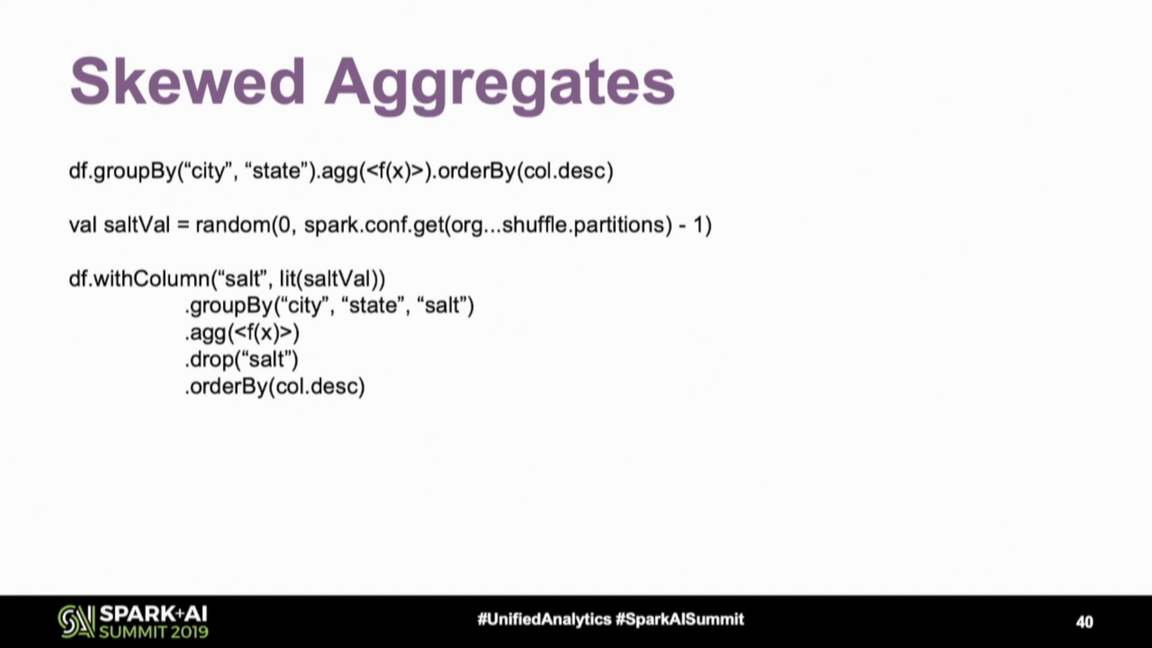
But keep in mind that you may need to combine the results afterward, so potentially execute another group by operation and introduce another shuffle. Check whether this extra shuffle won't be more expensive than a skewed partition.
Join
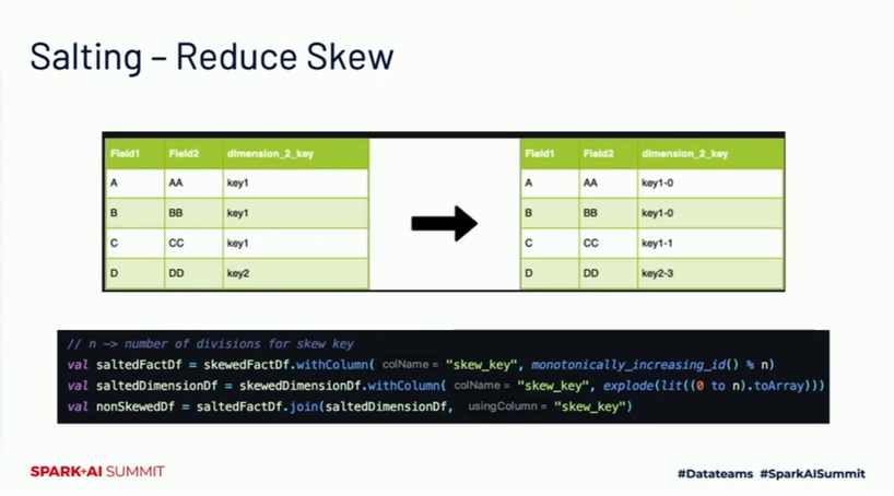
Other operations that can suffer from the skew are the joins. Here too, you can use the salting method and Blake Becerra pretty well explained it. The idea is to take the skewed DataFrame and improve the key distribution by adding the number from a finite set. After that, you have to explode the join column from the non-skewed DataFrame and add all possible numbers from the set so that the joins can still happen. Keep in mind that it will require a bit more memory since we're exploding the data - exactly as for input partitions sizing "unless use cases". Blake summarized this operation pretty well in the slide below:
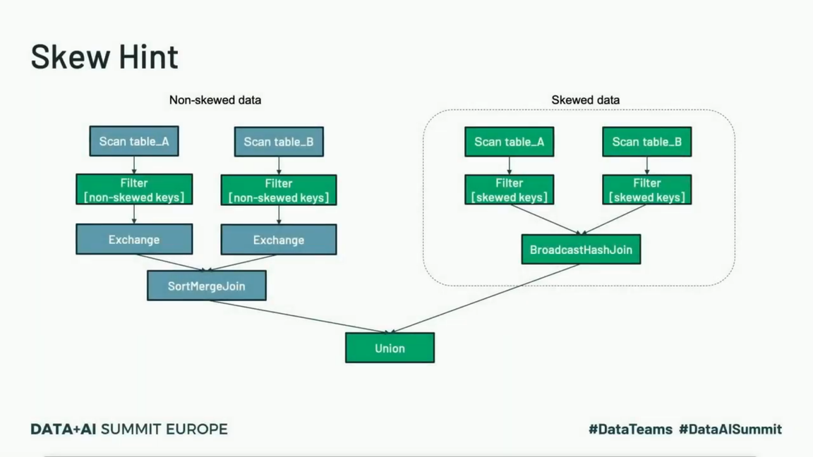
An alternative strategy was presented in the first Data+AI Summit edition by Suganthi Dewakar in the talk about skews management at PB scale at Facebook. This alternative requires some knowledge about the data and the skewed keys. Once identified, you have to split your query into 2, one for the skewed part, one for the rest, and UNION the result at the end. Thanks to that, there is more chance to use a more optimized broadcast join strategy and avoid data shuffle on the skewed side:
Suganthi also shared 2 other tips relying on the Adaptive Query Execution but since I'm trying to summarize here the "hard" tips, I invite you to watch it after, starting from 5:10.
Garbage Collector
Apache Spark runs on top of JVM, so you can also tune it with an appropriate Garbage Collection strategy. Blake's colleague from IBM, Kaushik Tadikonda, shared some tips about sizing and choosing the best Garbage Collection mode. If you use ParallelGC collection method and notice frequent minor GC, Kaushik recommends increasing Eden and Survivor Space. To handle frequently major GC in this mode, you can increase young space to prevent objects from being promoted to old space. You can also reduce the spark.memory.fraction property, but by doing that, you will probably spill more cached data to disk rather than keeping it in memory.
Regarding the G1GC collection, Kaushik recommends to use it for heaps greater than 8 GB and suffering from long GC times. You can also fine-tune some of the G1GC's properties like:
- ParallelGCThreads to the number of cores in the executor, let's say n
- ConcGC to the double of cores in the executor, n * 2
- InitiatingHeapOccupancyPercentage to 35 which will trigger GC when the 35% of the heap will be taken
But which of these 2 GC strategies should we choose? Rose Toomey shared some hints in her Spark+AI 2019 Europe talk. To put it simply, ParallelGC favors throughput, whereas G1GC is better suited for low latency for pipelines not operating on wide rows. In either way, you should always prefer frequent and early minor collections.
Cluster
Finally, the last part, and maybe the most expected, the cluster. Maybe I will deceive you, but I didn't find the talk saying, "use these parameters; it will work every time". The most often advice is more "start with this and iterate to improve". Because yes, performance tuning is an iterative process depending on various factors like the machine types, data organization, the volume to process, data location (same region than compute), and the job itself (remember Daniel's advice about partition sizes for data generation code).
Regarding the recommendations, Jean-Yves Stephan and Julien Dumazert recommend to set 4-8 cores per executor and the memory to 85% * (node memory / the number of executors per node). But it's not "the" configuration. It should be rather a baseline to tune.
Also, Daniel recalled essential points about the sizing. You should understand the hardware used to run your code. How much memory will you use per core? What disk (HDD, SSD?) will you work on? There are some throughput limitations on the data sources or data sinks, like the maximal number of simultaneous connections? And from more concrete recommendations, we can note the 70% threshold in Ganglia's load average metric representing the relationship between running and waiting to run processes.
One thing to keep in mind recalled by Kira Lindke is that changing one parameter impacts others. Too big executor memory may lead to excessive GCs; too small can slow down the processing, for example, with disk spilling.
We can optimize our workloads in different ways, and I hope you saw the confirmation for that in this blog post. It's not limited to the number of cores or memory available per core because they can be related to other parameters like partitions, GC configuration, and - especially - your code! If you have any other talks that I missed here, feel free to comment. The topic is so important that I think everybody will thank you for sharing!
Data Engineering Design Patterns

Looking for a book that defines and solves most common data engineering problems? I wrote
one on that topic! You can read it online
on the O'Reilly platform,
or get a print copy on Amazon.
I also help solve your data engineering problems contact@waitingforcode.com 📩
Read also about Performance optimization lessons from Spark+AI and Data+AI Summits here:
- Fine Tuning and Enhancing Performance of Apache Spark Jobs Apache Spark Core – Practical Optimization How Adobe Does 2 Million Records Per Second Using Apache Spark! Skew Mitigation For Facebook PetabyteScale Joins Apache Spark At Scale in the Cloud Fine Tuning and Enhancing Performance of Apache Spark Jobs How to Automate Performance Tuning for Apache Spark
Related blog posts:
- Rolling history logs in Spark History UI
- What's new in Apache Spark 3.4.0 - shuffle changes
- What's new in Apache Spark 3.4.0 - Spark Connect
In the new blog post I put together past #SparkAISummit and #DataAISummit talks about #ApacheSpark performance tips. If you want to watch them, all the links are in the introduction and below this blog post ? https://t.co/wfJT0t0hsO
— Bartosz Konieczny (@waitingforcode) February 20, 2021