
Apache Spark SQL provides advanced analytics features that we can find in more classical OLAP-based workloads. Below I'll explain one of them.
What would it take for you to trust your Databricks pipelines in production?
A 3-day bug hunt on a 3-person team costs up to €7,200 in lost engineering time. This workshop teaches you to prevent that — unit tests, data tests, and integration tests for PySpark and Databricks Lakeflow, including Spark Declarative Pipelines.

Konieczny
This post talks about grouping sets which represent cube and rollup operations. The first section starts by explaining grouping sets and comparing them to the classical GROUP BY operation. The next 2 parts show rollup and cube operators more in details. The last section focuses on the internal execution of multi-dimensional aggregations by taking rollup as an example.
Grouping sets
The most often used operation to aggregate data is GROUP BY. It's easy to understand but it has also an important drawback of rigidity - it always applies exclusively on specified columns:
WITH software_projects (country, language, projects_number) AS (
  SELECT 'pl' AS country, 'Scala' AS language, 10 AS projects_number UNION ALL SELECT 'pl' AS country, 'Java'  AS language, 1  AS projects_number UNION ALL SELECT 'pl' AS country, 'C++'  AS language, 2  AS projects_number
  UNION ALL
  SELECT 'us' AS country, 'Scala'  AS language, 15  AS projects_number UNION ALL SELECT 'us' AS country, 'Java'  AS language, 3  AS projects_number
  UNION ALL
  SELECT 'fr' AS country, 'Scala'  AS language, 5  AS projects_number UNION ALL SELECT 'fr' AS country, 'Java'  AS language, 9  AS projects_number
)

SELECT country, language, SUM(projects_number) FROM software_projects GROUP BY country, language;
 country | language | sum
---------+----------+-----
 us      | Scala    |  15
 pl      | C++      |   2
 pl      | Java     |   1
 fr      | Scala    |   5
 fr      | Java     |   9
 us      | Java     |   3
 pl      | Scala    |  10
(7 rows)
Above expression returns the sum of projects grouped by language and country. And it's fine in most of the cases. However, sometimes we may want to generate more complex aggregations. If we retake our example, we could wish for instance to get sums by country, (country, language) and exclusively by language. The naive approach would consist on writing 3 different queries and joining the results somehow (e.g. UNION). Fortunately, SQL comes with a built-in mechanism to deal with such a scenario. It's called GROUPING SETS. This feature lets us define groups on which given aggregation will be applied. In our case, we can define the groups for (country, language), (country) and (language) and get the aggregated results in a single query:
WITH software_projects (country, language, projects_number) AS (
  SELECT 'pl' AS country, 'Scala' AS language, 10 AS projects_number UNION ALL SELECT 'pl' AS country, 'Java'  AS language, 1  AS projects_number UNION ALL SELECT 'pl' AS country, 'C++'  AS language, 2  AS projects_number
  UNION ALL
  SELECT 'us' AS country, 'Scala'  AS language, 15  AS projects_number UNION ALL SELECT 'us' AS country, 'Java'  AS language, 3  AS projects_number
  UNION ALL
  SELECT 'fr' AS country, 'Scala'  AS language, 5  AS projects_number UNION ALL SELECT 'fr' AS country, 'Java'  AS language, 9  AS projects_number
)

SELECT country, language, SUM(projects_number) FROM software_projects
GROUP BY
    GROUPING SETS ((country, language), (country), (language));
 country | language | sum
---------+----------+-----
 us      | Scala    |  15
 pl      | C++      |   2
 pl      | Java     |   1
 fr      | Scala    |   5
 fr      | Java     |   9
 us      | Java     |   3
 pl      | Scala    |  10
 fr      |          |  14
 us      |          |  18
 pl      |          |  13
         | C++      |   2
         | Scala    |  30
         | Java     |  13
(13 rows)
Even though this section talks exclusively about SQL, it merits a small note about GROUPING SETS in Apache Spark SQL. This feature is not provided with DataFrame API. Instead, it's only supported with SQL mode. The API uses only rollup and cube detailed in next 2 section.
Rollup
Apache Spark SQL doesn't come with a programmatic support for grouping sets but it proposes 2 shortcut methods. One of them is rollup operator created from:
def rollup(cols: Column*): RelationalGroupedDataset
def rollup(col1: String, cols: String*): RelationalGroupedDataset
Rollup is a multi-dimensional aggregate operator, thus it applies specified aggregation on the grouping keys. The computation returns subtotals for n dimensions and a big total across the whole group. For instance, if we want to use the rollup on (key1, key2, key3), it will compute the subtotals for the combinations of following dimensions: (key1, key2, key3), (key1, key2) and (key1). The next example shows that pretty clearly:
  private val TestSparkSession = SparkSession.builder().appName("Spark grouping sets tests").master("local[*]")
    .getOrCreate()

  import TestSparkSession.implicits._

  private val Team1Label = "Team1"
  private val Team2Label = "Team2"

  private val TestedDataSet = Seq(
    ("pl", "Scala", Team1Label, 10), ("pl", "Java", Team1Label, 1), ("pl", "C++", Team2Label, 2),
    ("us", "Scala", Team2Label,15), ("us", "Java", Team2Label,3),
    ("fr", "Scala", Team2Label,5), ("fr", "Java", Team2Label,9)
  ).toDF("country", "language", "team", "projects_number")

  case class GroupingSetResult(country: String, language: String, team: String, aggregationValue: Long)

  private def mapRowToGroupingSetResult(row: Row) = GroupingSetResult(row.getAs[String]("country"),
    row.getAs[String]("language"), row.getAs[String]("team"), row.getAs[Long]("sum(projects_number)"))

  "rollup" should "compute aggregates by country, language and team" in {
    val rollupResults = TestedDataSet.rollup($"country", $"language", $"team").sum("projects_number")

    val collectedResults = rollupResults.collect().map(row => mapRowToGroupingSetResult(row)).toSeq

    collectedResults should have size 18
    collectedResults should contain allOf(
      GroupingSetResult("fr", "Java", "Team2", 9), GroupingSetResult("pl", "C++", "Team2", 2), GroupingSetResult("us", "Java", "Team2", 3),
      GroupingSetResult("fr", "Scala", "Team2", 5), GroupingSetResult("pl", "Java", "Team1", 1), GroupingSetResult("us", "Scala", "Team2", 15),
      GroupingSetResult("pl", "Scala", "Team1", 10),
      GroupingSetResult("pl", "Java", null, 1), GroupingSetResult("us", "Java", null, 3), GroupingSetResult("pl", "Scala", null, 10),
      GroupingSetResult("us", "Scala", null, 15), GroupingSetResult("fr", "Java", null, 9), GroupingSetResult("fr", "Scala", null, 5),
      GroupingSetResult("pl", "C++", null, 2),
      GroupingSetResult("pl", null, null, 13),GroupingSetResult("fr", null, null, 14), GroupingSetResult("us", null, null, 18),
      GroupingSetResult(null, null, null,45)
    )
    rollupResults.explain()
How does Apache Spark orchestrate the execution of rollup ? The physical execution plan for above code looks like:
== Physical Plan ==
      *(2) HashAggregate(keys=[country#42, language#43, team#44, spark_grouping_id#38], functions=[sum(cast(projects_number#12 as bigint))])
      +- Exchange hashpartitioning(country#42, language#43, team#44, spark_grouping_id#38, 200)
         +- *(1) HashAggregate(keys=[country#42, language#43, team#44, spark_grouping_id#38], functions=[partial_sum(cast(projects_number#12 as bigint))])
            +- *(1) Expand [List(projects_number#12, country#39, language#40, team#41, 0), List(projects_number#12, country#39, language#40, null, 1), List(projects_number#12, country#39, null, null, 3), List(projects_number#12, null, null, null, 7)], [projects_number#12, country#42, language#43, team#44, spark_grouping_id#38]
               +- LocalTableScan [projects_number#12, country#39, language#40, team#41]
As we can see, rollup is nothing more than an extended version of GROUP BY. It involves shuffle, so the data for the same key must be moved to the same executor. If we analyze the grouping keys carefully we can see the presence of a spark_grouping_id field. It represents the number corresponding to the bit vector of aggregated values. We'll see it more in details in the last section. For now, all you need to know is that each of grouping keys has an associated number and the combination is the sum of them.
Cube
If the rollup is an extension for group by, cube is an extension for rollup. Unlike earlier discussed operator, cube applies specified aggregation to all combinations of grouping keys. It means that for 3 columns we'll get the aggregation results for groups: (column1, column2, column3), (column1, column2), (column1, column3), (column1), (column2, column3), (column2), (column3) - exactly as in the test:
  "cube" should "compute aggregates by country, language and team" in {
    val cubeResults = TestedDataSet.cube($"country",  $"language", $"team").sum("projects_number")

    val collectedResults = cubeResults.collect().map(row => mapRowToGroupingSetResult(row)).toSeq

    collectedResults should have size 32
    collectedResults should contain allOf(
      // country, language, team
      GroupingSetResult("pl", "Scala", "Team1", 10), GroupingSetResult("fr", "Java", "Team2", 9), GroupingSetResult("pl", "C++", "Team2", 2),
      GroupingSetResult("us", "Java", "Team2", 3), GroupingSetResult("fr", "Scala", "Team2", 5), GroupingSetResult("pl", "Java", "Team1", 1),
      GroupingSetResult("us", "Scala", "Team2", 15),
      // country, language
      GroupingSetResult("us", "Java", null, 3), GroupingSetResult("pl", "Java", null, 1), GroupingSetResult("pl", "Scala", null, 10),
      GroupingSetResult("fr", "Java", null, 9), GroupingSetResult("fr", "Scala", null, 5), GroupingSetResult("us", "Scala", null, 15),
      GroupingSetResult("pl", "C++", null, 2),
      // country, team
      GroupingSetResult("us", null, "Team2", 18), GroupingSetResult("pl", null, "Team2", 2), GroupingSetResult("pl", null, "Team1", 11),
      GroupingSetResult("fr", null, "Team2", 14),
      // country
      GroupingSetResult("pl", null, null, 13), GroupingSetResult("us", null, null, 18), GroupingSetResult("fr", null, null, 14),
      // language, team
      GroupingSetResult(null, "Java", "Team2", 12), GroupingSetResult(null, "C++", "Team2", 2),
      GroupingSetResult(null, "Scala", "Team1", 10), GroupingSetResult(null, "Java", "Team1", 1), GroupingSetResult(null, "Scala", "Team2", 20),
      // language
      GroupingSetResult(null, "Scala", null, 30), GroupingSetResult(null, "Java", null, 13), GroupingSetResult(null, "C++", null, 2),
      // team
      GroupingSetResult(null, null, "Team1", 11),  GroupingSetResult(null, null, "Team2", 34),
      // total
      GroupingSetResult(null, null, null, 45)
    )
    cubeResults.explain()
  }
As you can see, the amount of generated results is much bigger than for rollup. However, the execution plan is not so much different:
== Physical Plan ==
*(2) HashAggregate(keys=[country#42, language#43, team#44, spark_grouping_id#38], functions=[sum(cast(projects_number#12 as bigint))])
+- Exchange hashpartitioning(country#42, language#43, team#44, spark_grouping_id#38, 200)
   +- *(1) HashAggregate(keys=[country#42, language#43, team#44, spark_grouping_id#38], functions=[partial_sum(cast(projects_number#12 as bigint))])
      +- *(1) Expand [List(projects_number#12, country#39, language#40, team#41, 0), List(projects_number#12, country#39, language#40, null, 1), List(projects_number#12, country#39, null, team#41, 2), List(projects_number#12, country#39, null, null, 3), List(projects_number#12, null, language#40, team#41, 4), List(projects_number#12, null, language#40, null, 5), List(projects_number#12, null, null, team#41, 6), List(projects_number#12, null, null, null, 7)], [projects_number#12, country#42, language#43, team#44, spark_grouping_id#38]
         +- LocalTableScan [projects_number#12, country#39, language#40, team#41]
Multi-dimensional aggregations execution
The physical plan already shows what happens under-the-hood. But if it's not clear, the following pictures should clarify that:
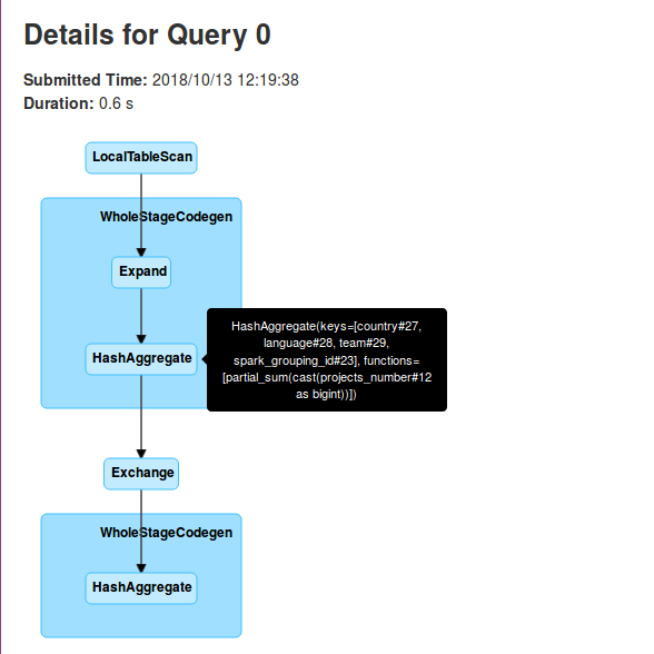
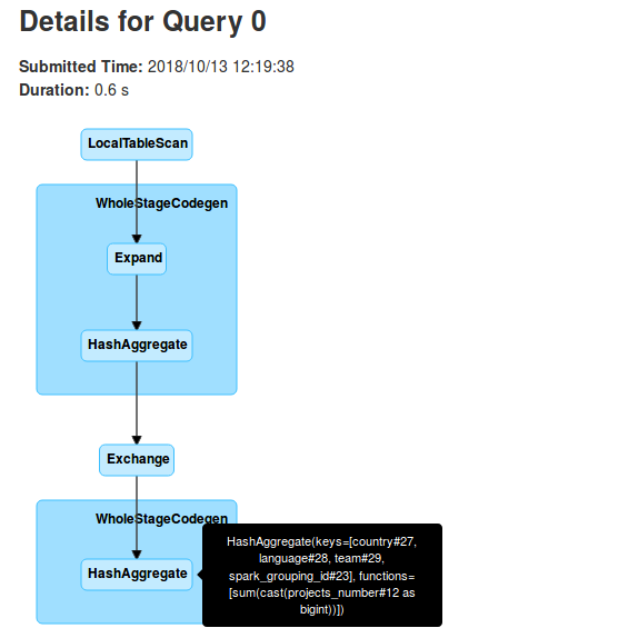
As you can see in above pictures, each executor does a partial aggregation locally on the initially received data. This partial execution is represented in the physical plan by:
HashAggregate(keys=[country#27, language#28, team#29, spark_grouping_id#23], functions=[partial_sum(cast(projects_number#12 as bigint))], output=[country#27, language#28, team#29, spark_grouping_id#23, sum#35L])
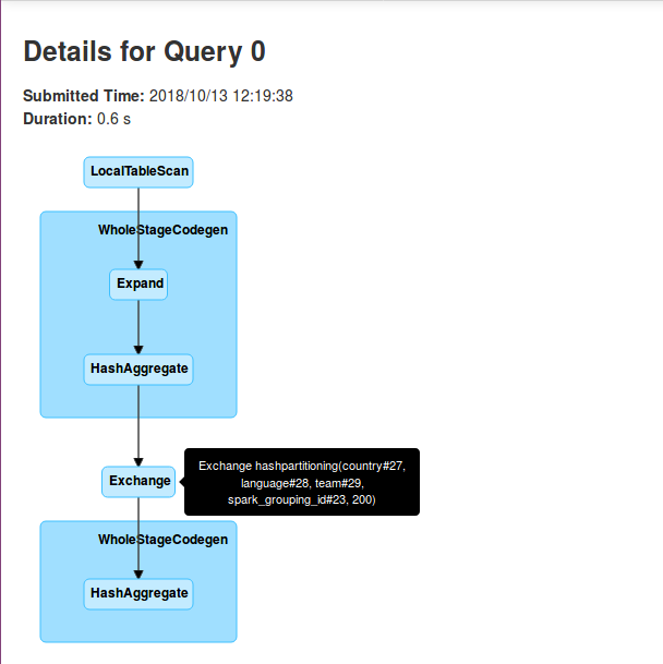
So in fact the grouping sets are more like RDD's reduce transformation. It also explains why the query executes 2 stages. The first one corresponds to partial aggregations and the second one to the final aggregation. And it's the latter stage that requires to shuffle the data accordingly to grouping keys assigned to the executors. And by the way, let's come back to these keys. In the second section I was talking about spark_grouping_id. It's a virtual column used to represent the columns used in the grouping set. The value for this column is computed from a bit mask which, in its turn, is based on the aggregation columns. We can see that by analyzing generated Java code:
/* 253 */   private void expand_doConsume(InternalRow inputadapter_row, int expand_expr_0, UTF8String expand_expr_1, boolean expand_exprIsNull_1, UTF8String expand_expr_2, boolean expand_exprIsNull_2, UTF8String expand_expr_3, boolean expand_exprIsNull_3) throws java.io.IOException {
/* 254 */     boolean expand_isNull1 = true;
/* 255 */     UTF8String expand_value1 = null;
/* 256 */     boolean expand_isNull2 = true;
/* 257 */     UTF8String expand_value2 = null;
/* 258 */     boolean expand_isNull3 = true;
/* 259 */     UTF8String expand_value3 = null;
/* 260 */     boolean expand_isNull4 = true;
/* 261 */     int expand_value4 = -1;
/* 262 */     for (int expand_i = 0; expand_i < 4; expand_i ++) {
/* 263 */       switch (expand_i) {
/* 264 */       case 0:
/* 265 */         expand_isNull1 = expand_exprIsNull_1;
/* 266 */         expand_value1 = expand_expr_1;
/* 267 */
/* 268 */         expand_isNull2 = expand_exprIsNull_2;
/* 269 */         expand_value2 = expand_expr_2;
/* 270 */
/* 271 */         expand_isNull3 = expand_exprIsNull_3;
/* 272 */         expand_value3 = expand_expr_3;
/* 273 */
/* 274 */         expand_isNull4 = false;
/* 275 */         expand_value4 = 0;
/* 276 */         break;
/* 277 */
/* 278 */       case 1:
/* 279 */         expand_isNull1 = expand_exprIsNull_1;
/* 280 */         expand_value1 = expand_expr_1;
/* 281 */
/* 282 */         expand_isNull2 = expand_exprIsNull_2;
/* 283 */         expand_value2 = expand_expr_2;
/* 284 */
/* 285 */         final UTF8String expand_value11 = null;
/* 286 */         expand_isNull3 = true;
/* 287 */         expand_value3 = expand_value11;
/* 288 */
/* 289 */         expand_isNull4 = false;
/* 290 */         expand_value4 = 1;
/* 291 */         break;
/* 292 */
/* 293 */       case 2:
/* 294 */         expand_isNull1 = expand_exprIsNull_1;
/* 295 */         expand_value1 = expand_expr_1;
/* 296 */
/* 297 */         final UTF8String expand_value14 = null;
/* 298 */         expand_isNull2 = true;
/* 299 */         expand_value2 = expand_value14;
/* 300 */
/* 301 */         final UTF8String expand_value15 = null;
/* 302 */         expand_isNull3 = true;
/* 303 */         expand_value3 = expand_value15;
/* 304 */
/* 305 */         expand_isNull4 = false;
/* 306 */         expand_value4 = 3;
/* 307 */         break;
/* 308 */
/* 309 */       case 3:
/* 310 */         final UTF8String expand_value17 = null;
/* 311 */         expand_isNull1 = true;
/* 312 */         expand_value1 = expand_value17;
/* 313 */
/* 314 */         final UTF8String expand_value18 = null;
/* 315 */         expand_isNull2 = true;
/* 316 */         expand_value2 = expand_value18;
/* 317 */
/* 318 */         final UTF8String expand_value19 = null;
/* 319 */         expand_isNull3 = true;
/* 320 */         expand_value3 = expand_value19;
/* 321 */
/* 322 */         expand_isNull4 = false;
/* 323 */         expand_value4 = 7;
/* 324 */         break;
/* 325 */       }
/* 326 */       ((org.apache.spark.sql.execution.metric.SQLMetric) references[9] /* numOutputRows */).add(1);
/* 327 */
/* 328 */       agg_doConsume(expand_expr_0, expand_value1, expand_isNull1, expand_value2, expand_isNull2, expand_value3, expand_isNull3, expand_value4);
/* 329 */
/* 330 */     }
/* 331 */
/* 332 */   }
/* 333 */
As you can see we have 4 grouping sets with the ids: 0, 1, 3 and 7. The first one applies when all columns are aggregated (country, language, team). The second id is used for 2 active columns (country, language) while the third to only one (country). The last id corresponds to global aggregation. We can deduce that from all 3 expand_valuens set to null. It's even more clear in the execution plan's Expand stage:
+- *(1) Expand [List(projects_number#12, country#24, language#25, team#26, 0), List(projects_number#12, country#24, language#25, null, 1), List(projects_number#12, country#24, null, null, 3), List(projects_number#12, null, null, null, 7)], [projects_number#12, country#27, language#28, team#29, spark_grouping_id#23]
Multi-dimensional aggregations are a powerful feature coming from data warehousing. Apache Spark provides a pretty efficient implementation of 2 aggregations of that type: rollup and cube. They use the idea of grouping sets and internally are executed as a reduce operation. Such implementation decreases the amount of shuffled data and helps to improve performances in this compute intensive operation.
Data Engineering Design Patterns

Looking for a book that defines and solves most common data engineering problems? I wrote
one on that topic! You can read it online
on the O'Reilly platform,
or get a print copy on Amazon.
I also help solve your data engineering problems contact@waitingforcode.com 📩
Read also about Grouping sets in Apache Spark SQL here:
Related blog posts:
#ApacheSpark #SparkSQL offers a lot of aggregations. Several of them are misknown - especially when you are coming to the data not from classical BI ground. Today I try to explain one of such aggregations called grouping sets (rollup and cube): https://t.co/EIcmF6iXZu
— Bartosz Konieczny (@waitingforcode) November 7, 2018