
Apache Spark has this great capacity to optimize joins of bucketed tables but does it work on partitions as well? No, and to understand why, I invite you to read the following sections of this blog post ?
What would it take for you to trust your Databricks pipelines in production?
A 3-day bug hunt on a 3-person team costs up to €7,200 in lost engineering time. This workshop teaches you to prevent that — unit tests, data tests, and integration tests for PySpark and Databricks Lakeflow, including Spark Declarative Pipelines.

Konieczny
The idea for this article born after an exchange I had on LinkedIn (👋 Pietro) where we're wondering whether it was possible - and if not - why, to use a partition-wise joins that do exist for example in Oracle. To address this question, the article is composed as follows. First, it presents the idea of a partition-wise join. Next, it tries to show how the bucket-based local joins work. The last part tries to answer why the partition-wise join is not present in Apache Spark and how it can be simulated.
A partition-aware join
Oracle is only one of databases supporting partitioning. And since it's a commercial solution, let's take an Open Source one like PostgreSQL to see what happens. To start, the tested partitioned tables look like that:
CREATE TABLE lower_case_letters (id INTEGER, letter VARCHAR(5)) PARTITION BY HASH (id);
CREATE TABLE upper_case_letters (id INTEGER, letter VARCHAR(5)) PARTITION BY HASH (id);

CREATE TABLE lower_case_letters_0 PARTITION OF lower_case_letters FOR VALUES WITH (MODULUS 2, REMAINDER 0);
CREATE TABLE lower_case_letters_1 PARTITION OF lower_case_letters FOR VALUES WITH (MODULUS 2, REMAINDER 1);
CREATE TABLE upper_case_letters_0 PARTITION OF upper_case_letters FOR VALUES WITH (MODULUS 2, REMAINDER 0);
CREATE TABLE upper_case_letters_1 PARTITION OF upper_case_letters FOR VALUES WITH (MODULUS 2, REMAINDER 1);


INSERT INTO lower_case_letters (id, letter) VALUES (1, 'A'), (100, 'AA'), (1000, 'AAA');
INSERT INTO upper_case_letters (id, letter) VALUES (1, 'A'), (100, 'AA'), (1000, 'AAA');
As you can see, we start by creating a "base" table. Later the PARTITION OF operator adds 4 partitioned tables. Every partition declaration follows with an operation managing row assignment to the given partition. In the example, you can see that it's the classical hash-based mod division algorithm putting even ids to the partition 0 and odd to the partition 1.
Let's see now how the execution plans look like. The first execution tree shows the plan for the disabled partition-wise join optimization (SET enable_partitionwise_join TO off):
test=# EXPLAIN SELECT * FROM lower_case_letters low JOIN upper_case_letters upp ON upp.id = low.id;
 Merge Join  (cost=460.55..1105.80 rows=42050 width=56)
   Merge Cond: (low.id = upp.id)
   ->  Sort  (cost=230.28..237.53 rows=2900 width=28)
         Sort Key: low.id
         ->  Append  (cost=0.00..63.50 rows=2900 width=28)
               ->  Seq Scan on lower_case_letters_0 low_1  (cost=0.00..24.50 rows=1450 width=28)
               ->  Seq Scan on lower_case_letters_1 low_2  (cost=0.00..24.50 rows=1450 width=28)
   ->  Sort  (cost=230.28..237.53 rows=2900 width=28)
         Sort Key: upp.id
         ->  Append  (cost=0.00..63.50 rows=2900 width=28)
               ->  Seq Scan on upper_case_letters_0 upp_1  (cost=0.00..24.50 rows=1450 width=28)
               ->  Seq Scan on upper_case_letters_1 upp_2  (cost=0.00..24.50 rows=1450 width=28)
What happens here? To recall, the plan should be read bottom-up. You can see that both tables are completely read and sorted by the join key. After that, the database engine performs the merge join. It's quite normal for a join operation. Does the plan with partition-wise join enabled look the same?
test=# EXPLAIN SELECT * FROM lower_case_letters low JOIN upper_case_letters upp ON upp.id = low.id;
 Append  (cost=201.28..837.53 rows=21024 width=56)
   ->  Merge Join  (cost=201.28..366.21 rows=10512 width=56)
         Merge Cond: (low_1.id = upp_1.id)
         ->  Sort  (cost=100.64..104.26 rows=1450 width=28)
               Sort Key: low_1.id
               ->  Seq Scan on lower_case_letters_0 low_1  (cost=0.00..24.50 rows=1450 width=28)
         ->  Sort  (cost=100.64..104.26 rows=1450 width=28)
               Sort Key: upp_1.id
               ->  Seq Scan on upper_case_letters_0 upp_1  (cost=0.00..24.50 rows=1450 width=28)
   ->  Merge Join  (cost=201.28..366.21 rows=10512 width=56)
         Merge Cond: (low_2.id = upp_2.id)
         ->  Sort  (cost=100.64..104.26 rows=1450 width=28)
               Sort Key: low_2.id
               ->  Seq Scan on lower_case_letters_1 low_2  (cost=0.00..24.50 rows=1450 width=28)
         ->  Sort  (cost=100.64..104.26 rows=1450 width=28)
               Sort Key: upp_2.id
               ->  Seq Scan on upper_case_letters_1 upp_2  (cost=0.00..24.50 rows=1450 width=28)
The partition-aware plan is different. As you can see, the merge join operation is performed directly at the partition level, which gives a bit more room for optimization like parallel execution of these parts. On the other side, it doesn't come without extra costs since it may require much more CPU time and memory.
Bucket-aware join recall
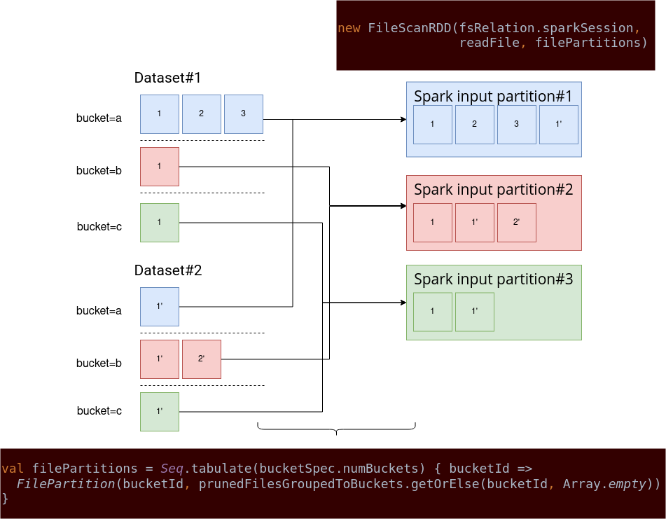
Can partition-wise join be implemented in Apache Spark? As you already know, Apache Spark can perform the bucket-wise joins without redistributing the data. To understand how the partition-wise join could work, let's explain first how the bucket-based join works. The RDD responsible for bucketed-data reads is FileScanRDD. Its constructor takes a sequence of FilePartition files that, as their name indicates, are the partitions:
class FileScanRDD(
    @transient private val sparkSession: SparkSession,
    readFunction: (PartitionedFile) => Iterator[InternalRow],
    @transient val filePartitions: Seq[FilePartition]) {
// ...
  override protected def getPartitions: Array[RDDPartition] = filePartitions.toArray
}
One of 2 places creating this RDD is createBucketedReadRDD method from FileSourceScanExec. Once again, the name is quite meaningful and helps to see the intent of this function. As you can deduce, it creates a "bucketed" version of the FileScanRDD. How? First, it groups all input files by bucket id. The bucket id is retrieved from every file because the bucket information is stored directly in the file name, always in the same place (after the last "_" and before the "c"). For example, in the part-00000-941bcfda-0876-413c-bee4-06bd691877d4_00001.c000.snappy.parquet file, the bucket number will be the "00001" part. After grouping the files, Apache Spark applies the bucket pruning optimization and transforms the outcome into a Seq[FilePartition] expected by the FileScanRDD.
A FilePartition instance stores the partition number and a list of files present on this partition:
case class FilePartition(index: Int, files: Array[PartitionedFile])
  extends Partition with InputPartition {
No surprise then, thanks to this operation, all files from a bucket are already located in the correct input partition. But it doesn't guarantee the absence of shuffle to perform the join operation of 2 same bucketed datasets. The no-shuffling guarantee is provided by the outputPartitioning attribute of the FileSourceScanExec. If the data source supports bucketing, the outputPartitioning will be the val partitioning = HashPartitioning(bucketColumns, spec.numBuckets). This snippet also shows how important it is to keep the same number of buckets for every dataset. Without that, the shuffle will still happen since the partition numbers won't be consistent!
The partitioning returned by the FileSourceScanExec is checked by EnsureRequirements:
    children = children.zip(requiredChildDistributions).map {
      case (child, distribution) if child.outputPartitioning.satisfies(distribution) =>
        child
      case (child, BroadcastDistribution(mode)) =>
        BroadcastExchangeExec(mode, child)
      case (child, distribution) =>
        val numPartitions = distribution.requiredNumPartitions
          .getOrElse(defaultNumPreShufflePartitions)
        ShuffleExchangeExec(distribution.createPartitioning(numPartitions), child)
    }
// org.apache.spark.sql.catalyst.plans.physical.Partitioning#satisfies
  final def satisfies(required: Distribution): Boolean = {
    required.requiredNumPartitions.forall(_ == numPartitions) && satisfies0(required)
  }
  protected def satisfies0(required: Distribution): Boolean = required match {
    case UnspecifiedDistribution => true
    case AllTuples => numPartitions == 1
    case _ => false
  }
For the case of bucket-based join, the first case will be satisfied, so it won't execute as a shuffle exchange. To sum up, since the input files are loaded to the same *input* partitions from the beginning, the step of redistributing the data to join won't be necessary.
What about partition-aware join?
Apache Spark knows that the bucket columns are involved in the join operation because of the metadata stored in the catalog. The catalog also contains the information about the columns used to partition the dataset for the ones written with partitionBy method. However, it doesn't use this information for data locality-based operations. I didn't find the references mentioning the whys, but IMHO, it comes from the conceptual difference between buckets and partitions. Buckets are known as "partitions of partitions", so they store smaller chunks of data. It means that the risk of memory problems when joining 2 buckets is smaller than doing the same for 2 bigger partitions (1 partition stores all buckets) at once. Partitioned joins would also decrease the parallelization level since we would have very few tasks processing big volumes of data (1 task per partition). If you have any input, I will be happy to learn!
If you want to perform partition-wise joins, you can try to simulate it with UNION operation, a bit like that:
  def listAllPartitions = Seq(0, 1, 2) // static for tests, but can use data catalog to get this info
  val partitionWiseJoins = listAllPartitions.map(partitionNumber => {
    // It's important to "push down" the partition predicate to make
    // the dataset smaller and eventually take advantage of small dataset
    // optimizations like broadcast joins
    val dataset1ForPartition = sparkSession.read.json(s"${dataset1Location}/partition_number=${partitionNumber}")
    val dataset2ForPartition = sparkSession.read.json(s"${dataset2Location}/partition_number=${partitionNumber}")
    dataset1ForPartition.join(dataset2ForPartition,
      dataset1ForPartition("order_id") === dataset2ForPartition("order_id"))
  })

  val unions = partitionWiseJoins.reduce((leftDataset, rightDataset) => leftDataset.unionAll(rightDataset))
  unions.explain(true)
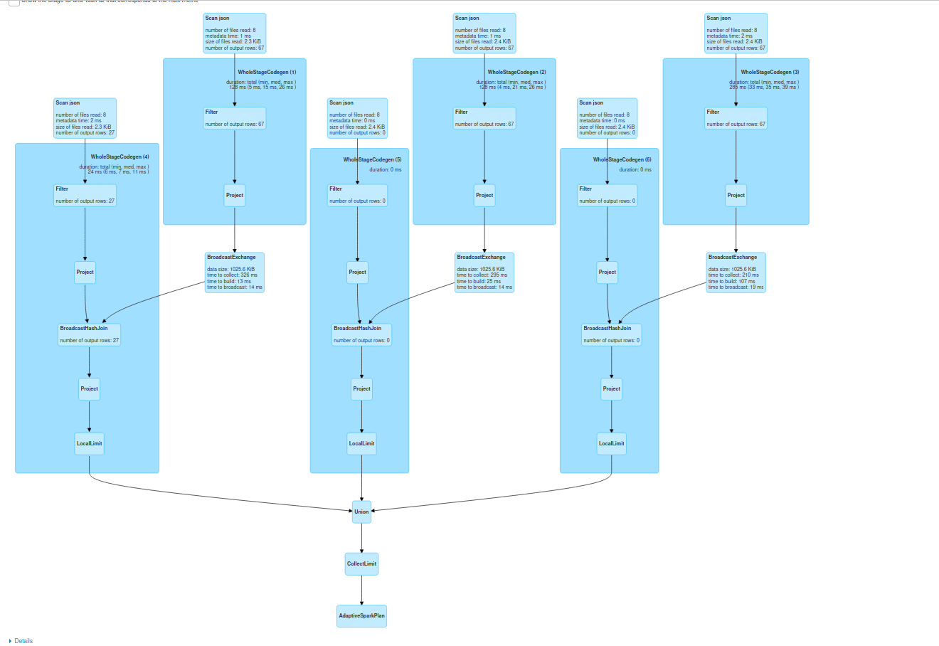
As you can see, the whole query comprises multiple, "partition-wise joins" which, if one partition is smaller, can be optimized to the local broadcast joins and returned as a single dataset after the union (UNION doesn't involve shuffle). But it's not a one-size-fits-all solution. For example, if the partition-wise joins are not optimized to the broadcast mode, the approach may not help in improving the performances. It won't also work when the potential joins can be located on different partitions. However, the last point is by definition not included in the partition-wise joins idea (see how the partitioned tables are defined in PostgreSQL's snippet from the first section). In the following picture you can see the execution plan for the partition-wise join simulation showing one broadcasted side in the joins:
To summarize, even though Apache Spark doesn't include the partition-wise optimization, it does include the bucket-based one to perform the local joins. But it doesn't mean you shouldn't try to optimize your non-bucketed code! As you saw in the last part, the UNION operator of the partitioned datasets is one of the possible approaches. It does not guarantee better results, but it's worth giving a try if you cannot reorganize your dataset to take advantage of the bucket-based joins and when you feel that it can improve the operation.
Data Engineering Design Patterns

Looking for a book that defines and solves most common data engineering problems? I wrote
one on that topic! You can read it online
on the O'Reilly platform,
or get a print copy on Amazon.
I also help solve your data engineering problems contact@waitingforcode.com 📩
Read also about Partition-wise joins and Apache Spark SQL here:
Related blog posts:
Partition-wise joins concept exists in different RDBMS. In my new article you can see its example in #PostgreSQL and discover whether it exists in #ApacheSpark #SparkSQL ? https://t.co/tRResH3Vf3
— Bartosz Konieczny (@waitingforcode) November 29, 2020