
A query adapting to the data characteristics discovered one-by-one at runtime? Yes, in Apache Spark 3.0 it's possible thanks to the Adaptive Query Execution!
What would it take for you to trust your Databricks pipelines in production?
A 3-day bug hunt on a 3-person team costs up to €7,200 in lost engineering time. This workshop teaches you to prevent that — unit tests, data tests, and integration tests for PySpark and Databricks Lakeflow, including Spark Declarative Pipelines.

Konieczny
I will deep delve into the AQE optimizations in my next blog posts. Here I'll present this feature from a general perspective, proving why it's...adaptive :) In the first part, you'll discover then the global presentation of the idea. After that, you will see different use cases tested by the community before the official implementation in Apache Spark codebase (!). Finally, in the next parts, you will see some implementation details and an example of the query optimized with the AQE feature.
Big picture
Apache Spark, and data processing frameworks in general, doesn't know the data itself before starting the processing. Well, they can define the overall dataset size, sometimes estimate the partition size if it's explicitly used (custom partitioner, partitioned data source with statistics), eventually use the metadata from the catalog if the latter exists and can be applied, but generally, they don't know a lot about the data produced in the processing logic. In consequence, the jobs can deal with different processing anomalies, like data skews where the size of one partition is much bigger than the others.
In simple and more Spark-centric terms, Adaptive Query Execution is a way to optimize the execution plan after performing the map stage tasks. For example, if after a map-filter operation of 2 joined Datasets, the engine sees that one of the filtered sides of the join is very small, it can decide to broadcast it instead of shuffling the data.
Adaptive Query Execution is then a possibility to change the execution plan at runtime, regarding the dataset characteristics (hence adaptive).
Examples
In the previous section I already gave you an example of such optimization. But using a broadcast join strategy instead of a shuffle strategy is only one of the examples. Another one, still related to the size of the data after the map stage, addresses the number of the reduce tasks. Thanks to that, the engine can decide whether a lot of small partitions should be merged into fewer smaller ones (coalesce shuffle partitions) to improve the performance.
Another feature of the AQE is the possibility to deal with data skews. If for whatever reason a partition of one join side is much bigger than the other partitions, Apache Spark can decide to subdivide it into smaller parts to increase the execution parallelism.
Internals - InsertAdaptiveSparkPlan
All the magic happens in InsertAdaptiveSparkPlan plan optimization rule. When called, the rule uses spark.sql.adaptive.enabled configuration flag to detect whether the query should be adaptive or not:
  override def apply(plan: SparkPlan): SparkPlan = applyInternal(plan, false)

  private def applyInternal(plan: SparkPlan, isSubquery: Boolean): SparkPlan = plan match {
    case _ if !conf.adaptiveExecutionEnabled => plan
    case _: ExecutedCommandExec => plan
    case c: DataWritingCommandExec => c.copy(child = apply(c.child))
    case c: V2CommandExec => c.withNewChildren(c.children.map(apply))
    case _ if shouldApplyAQE(plan, isSubquery) =>
As you can notice, the AQE will not be applied everywhere. Apart from the explicit cases, mostly related to the data writing, there is a shouldApplyAQE method that verifies some other criteria:
- spark.sql.adaptive.forceApply flag set to true - to force the AQE execution
- the query contains some Exchange nodes that represent the shuffle or broadcast events
- the query contains some subqueries
- the analyzed node is a subquery
When one of these conditions is met, another verification is performed which can invalidate the AQE applying. Inside it, Apache Spark verifies for all nodes of the plan:
- logical plan link presence - the physical plan is linked with its initial logical plan that is later used in the Adaptive Query Execution to transform it into the format understandable by the AQE (LogicalQueryStage for all stages that need to be optimized
- logical plan characteristics - a streaming query and dynamic pruning subquery are not supported
The result of this physical optimization is a AdaptiveSparkPlanExec node containing:
- initial physical plan - it will be used later to initialize the currentPhysicalPlan that will change at every adaptive execution in the node:
@volatile private var currentPhysicalPlan = applyPhysicalRules(initialPlan, queryStagePreparationRules) - an AdaptiveExecutionContext instance used to bring SparkSession to the node and cache to track duplicated Exchanges (if spark.sql.exchange.reuse is true)
- preprocessing rules like PlanAdaptiveSubqueries. InsertAdaptiveSparkPlan will be applied to all subquery nodes of the initial plan via this method:
  def compileSubquery(plan: LogicalPlan): SparkPlan = {
    // Apply the same instance of this rule to sub-queries so that sub-queries all share the
    // same `stageCache` for Exchange reuse.
    this.applyInternal(
      QueryExecution.createSparkPlan(adaptiveExecutionContext.session,
        adaptiveExecutionContext.session.sessionState.planner, plan.clone()), true)
  }
If one of the subquery nodes doesn't support adaptive execution (already mentioned verifications), the optimization will fall back to the not adaptive execution plan. - subquery flag to control UI notifications (UI doesn't support partial updates yet; for subquery, only SQL metrics for new plan nodes will be updated)
If everything can be dynamically optimized, the physical optimization happens.
Internals - AdaptiveSparkPlanExec
What happens then during the physical execution? First, Apache Spark creates the initial version of the new plan from the starting physical plan. It does it in createQueryStages(plan: SparkPlan) method and the outcome of this operation is an instance of CreateStageResult(newPlan: SparkPlan, allChildStagesMaterialized: Boolean, newStages: Seq[QueryStageExec])). This createQueryStages method is called every time the plan changes, so let's stop a little and focus on it.
The createQueryStages recursively applies bottom-up on all the nodes of the physical plan passed in parameter. The transformation is different according to the node type:
- for an Exchange type, the Exchange node is replaced by a QueryStageExec node, ShuffleQueryStageExec for shuffle exchange or BroadcastQueryStageExec for the broadcast one
- for a QueryStageExec type,
- for remaining types, the createQueryStages function is applied on the direct children of the node, which of course can lead to another call of createQueryStages and creation of other QueryStageExec instance
The returned CreateStageResult is used later in this loop, as long as not all its children stages are computed:
      while (!result.allChildStagesMaterialized) {
        currentPhysicalPlan = result.newPlan
// ... execute the missing stages
        // Now that some stages have finished, we can try creating new stages.
        result = createQueryStages(currentPhysicalPlan)
}
As you can see, the CreateStageResult is updated every time a QueryStageExec completes, so when the broadcast or shuffle happens. When this moment is reached, the new statistics are available and can be used to create a new cheaper plan, that will be promoted to the current plan:
        val logicalPlan = replaceWithQueryStagesInLogicalPlan(currentLogicalPlan, stagesToReplace)
        val (newPhysicalPlan, newLogicalPlan) = reOptimize(logicalPlan)
        val origCost = costEvaluator.evaluateCost(currentPhysicalPlan)
        val newCost = costEvaluator.evaluateCost(newPhysicalPlan)
        if (newCost < origCost ||
            (newCost == origCost && currentPhysicalPlan != newPhysicalPlan)) {
          logOnLevel(s"Plan changed from $currentPhysicalPlan to $newPhysicalPlan")
          cleanUpTempTags(newPhysicalPlan)
          currentPhysicalPlan = newPhysicalPlan
          currentLogicalPlan = newLogicalPlan
          stagesToReplace = Seq.empty[QueryStageExec]
        }
The new plan is built from this optimizer instance that for now (3.0.0) supports only one optimization that adds a no-broadcast-hash-join hint when one join side has a lot of empty partitions:
  // The logical plan optimizer for re-optimizing the current logical plan.
  @transient private val optimizer = new RuleExecutor[LogicalPlan] {
    // TODO add more optimization rules
    override protected def batches: Seq[Batch] = Seq(
      Batch("Demote BroadcastHashJoin", Once, DemoteBroadcastHashJoin(conf))
    )
  }
If the new plan has a smaller cost than the previous one, it's promoted to the current plan and will be optimized in its turn in the introduced while loop. But wait a minute, where are these all skew and coalesce optimizations I quoted before? They're invoked twice. The first place is when a new query strage is created:
  private def newQueryStage(e: Exchange): QueryStageExec = {
    val optimizedPlan = applyPhysicalRules(e.child, queryStageOptimizerRules)
    val queryStage = e match {
      case s: ShuffleExchangeExec =>
        ShuffleQueryStageExec(currentStageId, s.copy(child = optimizedPlan))
      case b: BroadcastExchangeExec =>
        BroadcastQueryStageExec(currentStageId, b.copy(child = optimizedPlan))
    }
    currentStageId += 1
    setLogicalLinkForNewQueryStage(queryStage, e)
    queryStage
  }
As you can see, there is a queryStageOptimizerRules field that helps to create a new plan for every exchange. The second place where these optimizations are applied is here:
      // Run the final plan when there's no more unfinished stages.
      currentPhysicalPlan = applyPhysicalRules(result.newPlan, queryStageOptimizerRules)
      isFinalPlan = true
      executionId.foreach(onUpdatePlan(_, Seq(currentPhysicalPlan)))
      currentPhysicalPlan
It's the snippet from the previously analyzed getFinalPhysicalPlan method, executed after the while (!result.allChildStagesMaterialized) { loop, so when all stages intermediate stages are finished.
Example illustration
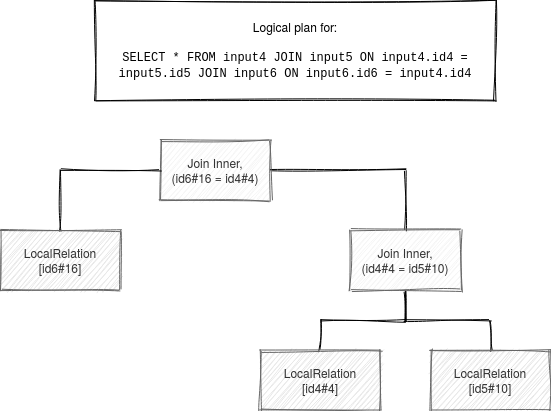
To analyze what happens when the Adaptive Query Execution is enabled, let's take the following query:
SELECT * FROM input4 JOIN input5 ON input4.id4 = input5.id5 JOIN input6 ON input6.id6 = input4.id4
The first logical plan looks like in the following schema:
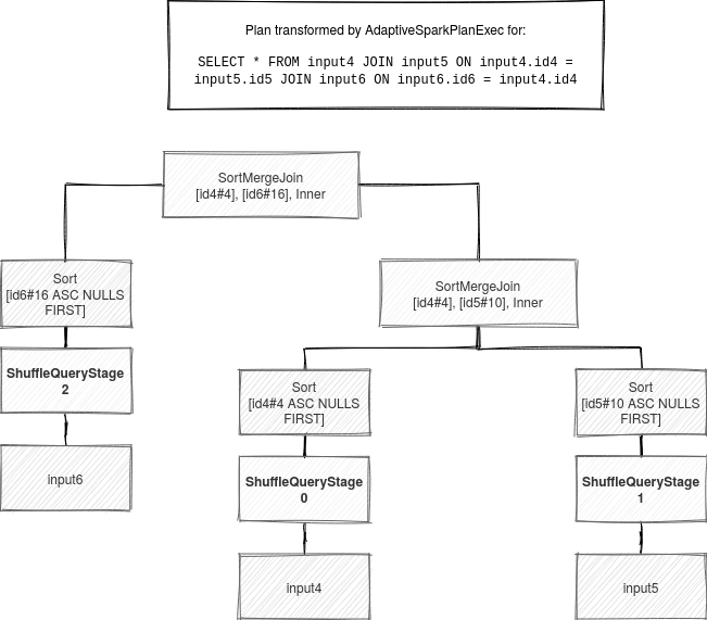
When the AQE starts, AdaptiveSparkPlanExec first transforms these nodes into a tree containing query stages:
After the first transformation, the algorithm remembers all new and not resolved query stages:
newStages = {$colon$colon@8691} "::" size = 3
 0 = {ShuffleQueryStageExec@11581} "ShuffleQueryStage 0\n+- Exchange hashpartitioning(id4#4, 200), true, [id=#43]\n   +- LocalTableScan [id4#4]\n"
 1 = {ShuffleQueryStageExec@11582} "ShuffleQueryStage 1\n+- Exchange hashpartitioning(id5#10, 200), true, [id=#49]\n   +- LocalTableScan [id5#10]\n"
 2 = {ShuffleQueryStageExec@11583} "ShuffleQueryStage 2\n+- ReusedExchange [id6#16], Exchange hashpartitioning(id5#10, 200), true, [id=#49]\n"
The stages are later submitted for the physical execution in that snippet:
          result.newStages.foreach { stage =>
            try {
              stage.materialize().onComplete { res =>
                if (res.isSuccess) {
                  events.offer(StageSuccess(stage, res.get))
                } else {
                  events.offer(StageFailure(stage, res.failed.get))
                }
              }(AdaptiveSparkPlanExec.executionContext)
            } catch {
              case e: Throwable =>
                cleanUpAndThrowException(Seq(e), Some(stage.id))
            }
          }
        }
Since the stages are created bottom-up, the first submitted stages will be the leaf nodes (no child query stages). The parent stages will then execute only when their children stages finish. As soon as one stage is available (= computed), the algorithm is notified and the outcome validation is performed:
        val nextMsg = events.take()
        val rem = new util.ArrayList[StageMaterializationEvent]()
        events.drainTo(rem)
        (Seq(nextMsg) ++ rem.asScala).foreach {
          case StageSuccess(stage, res) =>
            stage.resultOption = Some(res)
          case StageFailure(stage, ex) =>
            errors.append(ex)
        }

        // In case of errors, we cancel all running stages and throw exception.
        if (errors.nonEmpty) {
          cleanUpAndThrowException(errors, None)
        }
Next, in the current active logical plan, all query stages are replaced by LogicalQueryStages wrapping the initial logical node and corresponding physical node. After this step, the plan looks like:
Join Inner, (id6#16 = id4#4)
:- Join Inner, (id4#4 = id5#10)
:  :- LogicalQueryStage LocalRelation [id4#4], ShuffleQueryStage 0
:  +- LogicalQueryStage LocalRelation [id5#10], ShuffleQueryStage 1
+- LogicalQueryStage LocalRelation [id6#16], ShuffleQueryStage 2
So transformed plan has new statistics available and is later reoptimized, which can result in a completely new, pragmatic-based, plan:
val (newPhysicalPlan, newLogicalPlan) = reOptimize(logicalPlan)
And the costs of the old and new plans are compared:
        val origCost = costEvaluator.evaluateCost(currentPhysicalPlan)
        val newCost = costEvaluator.evaluateCost(newPhysicalPlan)
        if (newCost < origCost ||
            (newCost == origCost && currentPhysicalPlan != newPhysicalPlan)) {
          logOnLevel(s"Plan changed from $currentPhysicalPlan to $newPhysicalPlan")
          cleanUpTempTags(newPhysicalPlan)
          currentPhysicalPlan = newPhysicalPlan
          currentLogicalPlan = newLogicalPlan
          stagesToReplace = Seq.empty[QueryStageExec]
        }
        // Now that some stages have finished, we can try creating new stages.
        result = createQueryStages(currentPhysicalPlan)
And as you can see, if the new optimized plan is more optimal than the previous one, it's promoted as the new currentPhysicalPlan and currentLogicalPlan. Once all query stages are executed, the final physical plan is generated:
      currentPhysicalPlan = applyPhysicalRules(result.newPlan, queryStageOptimizerRules)
      isFinalPlan = true
      executionId.foreach(onUpdatePlan(_, Seq(currentPhysicalPlan)))
      currentPhysicalPlan
It was just an introduction. The Adaptive Query Execution is a more wide topic, difficult to explain in a single post. That's why in the next ones you can expect some more details about the specific optimizations resulting from the adaptive physical plan.
Data Engineering Design Patterns

Looking for a book that defines and solves most common data engineering problems? I wrote
one on that topic! You can read it online
on the O'Reilly platform,
or get a print copy on Amazon.
I also help solve your data engineering problems contact@waitingforcode.com 📩
Read also about What's new in Apache Spark 3.0 - Adaptive Query Execution here:
Related blog posts:
- What's new in Apache Spark 3.0 - Kubernetes
- What's new in Apache Spark 3.0 - GPU-aware scheduling
- What's new in Apache Spark 3 - Structured Streaming
- What's new in Apache Spark 3.0 - UI changes
- What's new in Apache Spark 3.0 - dynamic partition pruning
A query that adapts to the data during the execution? Sounds like JIT compiler but it's Adaptive Query Execution, another new feature of #ApacheSpark #SparkSQL. Curious about it? The first post of the series is online https://t.co/1vcM8TW524
— Bartosz Konieczny (@waitingforcode) July 25, 2020