
You know me already. I like to compare things to spot some differences and similarities. This time, I will do this exercise for cloud data warehouses, AWS Redshift, and Azure Synapse Analytics.
What would it take for you to trust your Databricks pipelines in production?
A 3-day bug hunt on a 3-person team costs up to €7,200 in lost engineering time. This workshop teaches you to prevent that — unit tests, data tests, and integration tests for PySpark and Databricks Lakeflow, including Spark Declarative Pipelines.

Konieczny
Architecture
At first glance, one could think that both data warehouses are completely different but in fact, both rely on the Massively Parallel Processing architecture pattern. In a nutshell, there is a node responsible for getting user query and generating the execution plan. Later, it passes the generated plan for the physical execution to the compute nodes that may exchange any intermediary data via a service bus. Please notice that I'm talking about Redshift and Dedicated SQL Pool and not about other components of these services.
But it can be a good moment to explain these services too! In addition to the Dedicated SQL Pool, Synapse also has Serverless Pool component. You can use it to read the external tables created on Blob Storage or Data Lake Gen 2. Since it's a serverless solution, it's very flexible, and you don't need to manage the hardware. Redshift has a similar serverless component called Redshift Spectrum. As for Serverless Pool, you can use it to read your objects from S3. The difference is the number of supported formats. While Spectrum supports both structured (Parquet, Avro, ORC, ...) and semi-structured (JSON, CSV, ...) formats, Serverless Pool only supports Parquet, CSV, and JSON files.
Loading data
We know already what we can do and in what mode, but any data warehouse will be useless without the data! So, how can we bring the data into them? For AWS Redshift, you can use a COPY method to load one or multiple files from your S3 bucket simultaneously. The operation has some important options like schema mapping, errors management, or data conversion. It also can load the data from DynamoDB. Regarding Synapse, it also has a COPY method, with similar features (errors management, compression). The difference is that Synapse's COPY supports only JSON, CSV, and Parquet, while Redshift's one can also handle the ORC columnar format. Also, Synapse's COPY works only with Blob Storage and Data Lake Gen 2. There is no connector for CosmosDB, although there is a way to work on CosmosDB data with the Synapse Link feature that creates CosmosDB's copy dedicated for Synapse analytical queries.
In Synapse, a popular alternative for COPY is PolyBase that favors the ELT approach. It creates an external table on Blob Storage or Data Lake Gen 2 that you can load directly to the Dedicated Pool with SQL.
Data layout
And what happens once we've loaded the data? Since both solutions are distributed, we need to think about organizing the data. Hopefully, Synapse and Redshift share the same data distribution methods which are:
- hash (Synapse), key (Redshift) - rows with the same key(s) defined in the hash/key distribution are stored together so that in any shuffle operation like joins or group bys, the engine doesn't need to move the data
- replicated (Synapse), all (Redshift) - good choice for small and not frequently updated tables. The engine replicates the whole table in every node.
- round-robin (Synapse), even (Redshift) - good strategy when you don't know the query patterns or want to load the data into a staging table. It distributes the records evenly so that every node gets approximately the same volume of data.
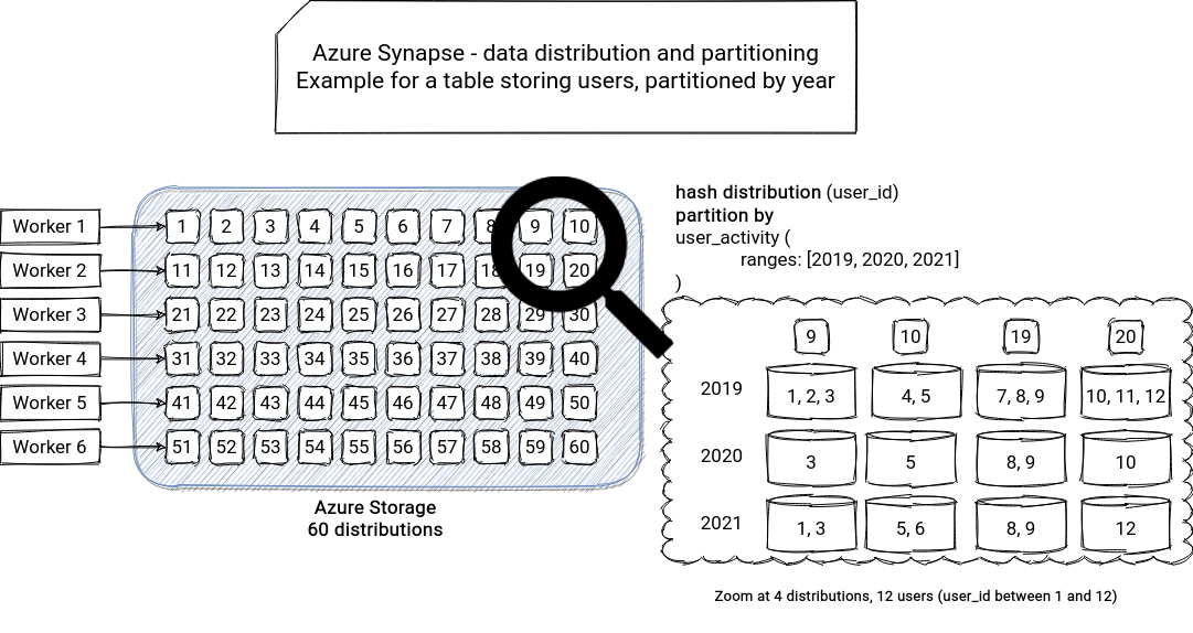
Of course, if we analyzed the data model only with this data distribution aspect, it would be too easy. Unfortunately, it's not the single aspect. In Synapse, you can also use partitions and indexes. It took me a while to understand the difference, so let me share it here. Synapse stores a distributed table across 60 distributions. It concerns the round-robin and hash distribution strategies because the replicated is stored on the compute node. Let's take an example of a hash-distributed table. If the table is also partitioned, each distribution will be responsible for distinct partitions. Put another way, the partitions will be distributed. Below you can find an example of a hash-distributed table on a user_id column, partitioned by user_activity date:
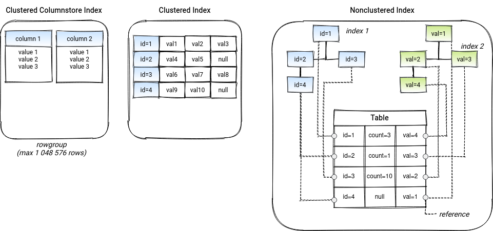
In addition to the distributions, Synapse also has a concept of indexes, which is not obvious too! By default, Synapse with create a Clustered Columnstore Index (CCI). It's composed of a rowgroup where Synapse stores table data in a column-oriented storage. It can then rely on column compression to optimize the storage and querying (segment skipped if it doesn't contain relevant data to the query). Large tables with more than 100 million rows can take full advantage of the compression. The CCI can also be ordered to ensure that every segment contains a not overlapping subset of data meaning that it will be either fully skipped or read. That's why it's good to use this ordering column in the filtering expressions of the query.
Another type of supported index is Clustered Index that stores data rows ordered by the index key. It's good for queries targeting a specific value or a small range of values or tables up to 100 million rows (e.g., dimension tables). You can also create a nonclustered index as an extra filter optimization strategy on top of a clustered index. To terminate, you can also use Heap tables which don't have any special indexing purposes and are then good candidates for staging data because data loading performs faster. The picture below summarizes the indexes categories:
And what about Redshift data layout? It stores data in columns. Each column can have multiple 1MB blocks with the data. Every block has a metadata layer storing at least the min and max values present in the block. This metadata layer will be useful to skip the blocks not relevant to the query predicate. But, exactly like in Synapse, these blocks can be less efficient if the table isn't sorted. That's why Redshift supports the sort key attribute, which defines the order for the rows stored in the blocks, a little bit like the ordered columnstore index in Synapse. The sort key is a great way to optimize range queries because the engine can easily skip the blocks not relevant to the query condition.

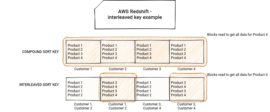
The sort key can be a simple key, a compound key which is composed of multiple columns, or an interleaved key which gives the same weight for all columns in the key. The interleaved key is optimized for the queries filtering on one or multiple columns of the key. How? Let's imagine the situation presented in the picture below. Customer id and product id are used in the sort key. For the sake of simplicity, let's assume that we have the blocks of 4 items each. With a standard compound key, the block stores all items of one customer and the queries involving only the customer id will be efficient. But it won't happen for the ones with product id because the product id column is considered as a secondary sort key, used only to order the products within a customer. The interleaved key assigns the same importance for each key meaning that the data will be organized differently. Thanks to it, querying for a product id can skan only 2 blocks instead of 4!
Security
The security part is also important. To start, let's focus on data safety. Both services support encryption at rest and encryption in transit but with few subtle differences. Synapse encrypts data at rest by default with the service-managed keys. You can also extend it with the Bring Your Own Key feature and manage the encryption keys alone. Redshift also supports customer-managed encryption with a similar backed service (KeyVault for Synapse, KMS for Redshift). However, Redshift doesn't encrypt your data by default with a kind of service-managed key.
Regarding other part of data, the data access, Synapse and Redshift support column-level security with SQL's GRANT operation. Both also provide a way to implement a row-level security strategy but through a different mechanism. Synapse does it with security policy which is a function predicate associated with a table and filtering rows on a user's identity based condition. Redshift supports the row-level security feature with views extending their WHERE clause by the condition based on the user's identity.
Another security part is the data loss protection. Very often, this feature is implemented with the system of backups. Synapse and Redshift support automated and manual backups, and both share very similar pros and cons. The cluster manages the automated snapshots, so you don't have anything to do. But it comes with some extra costs like a limited retention period. Regarding the manual snapshots, they're the snapshots explicitly taken by you, involving a proper triggering and monitoring mechanism. However, in Redshift, they're not deleted automatically, so that you can use them as a protection against cluster deletion! It's not the case in Synapse where they are retained only for 7 days. A possibility to extend this period is still under discussion.
And let's terminate this part with the network isolation. Regarding Azure Synapse, you can isolate it in 2 different ways. Either by managing the VNet on your own or by using the managed VNet feature. In addition to that, you can also benefit from the Managed Private Endpoint to enable communication with other Azure services exclusively via the Azure network. Redshift also supports private network traffic in place of public and internet-based traffic, with the feature called VPC enhanced routing. And regarding the VPC management, apparently, there is no similar managed option, but you can still isolate your cluster from the other parts of your system with the VPC managed by you.
Concurrency, scaling, elasticity
To terminate this article, let's focus on the day-to-day use and one of the most challenging dangers, peak loads. To handle any extra load in Redshift, you can simply resize the cluster. Currently, the solution supports 2 resizing modes, the classic and elastic. The first mode is faster, but it doesn't apply to all configurations, and whenever the configuration is not supported, you have to choose the classic mode. In both cases, the original cluster remains in the read-only mode.
But scaling a cluster is not a single option available in Redshift. You can also use a feature called concurrency scaling, which adds an extra compute power to the cluster dynamically. It's a part of a wider concept called Workload Management.
That was for Redshift, but what can we do with Synapse? You can also scale your cluster but not by changing its hardware composition. Instead, you have to change the number of associated Data Warehouse Units (DWU). A DWU is a combination of CPU, memory, and IO, so 3 important factors impacting query performance and the association of distributions; DWUs with a bigger number of nodes are responsible for more distributions than the smaller ones. Since the storage is decoupled from the compute, changing DWU doesn't have an impact on it. Synapse also supports workload management but without the automatic concurrency scaling option.
How does Synapse share the resources? It uses a concept called resource class. It defines the compute resources allocated for each user running a query. For example, a resource class called staticrc10 allocated 1 concurrency slot by user if the DW100c unit is configured in the cluster (BTW, the "unit's" correct name is Service Level). If you assign a staticrc30 class, the user will use 4 concurrency slots. That's for the
To not write a book, I decided to focus on the aforementioned 5 aspects in the comparison. You can see that despite some subtle differences, we can find similar concepts in both data warehouses.
Data Engineering Design Patterns
Looking for a book that defines and solves most common data engineering problems? I wrote
one on that topic! You can read it online
on the O'Reilly platform,
or get a print copy on Amazon.
I also help solve your data engineering problems contact@waitingforcode.com 📩
Read also about AWS Redshift vs Azure Synapse Analytics here:
- Azure Synapse Analytics - James Serra - SQLBits 2020 Guidance for designing distributed tables using dedicated SQL pool in Azure Synapse Analytics Cheat sheet for dedicated SQL pool (formerly SQL DW) in Azure Synapse Analytic Azure Synapse Analytics : Choose Right Index and Partition (Dedicated SQL Pools)
Related blog posts:
- What's new on the cloud for data engineers - part 12 (10.2023-02.2024)
- Vertical autoscaling for data processing on the cloud
- What's new on the cloud for data engineers - part 11 (06-09.2023)
Four months ago I compared BigQuery with Redshift. Today I repeated this exercise but this time for Redshift and Synapse ? https://t.co/0rObdyoiru
— Bartosz Konieczny (@waitingforcode) July 11, 2021