
I wrote this blog post a week before passing the GCP Data Engineer exam, hoping it'll help to organize a few things in my head (it did!). I also hope that it'll help you too in understanding ML from a data engineering perspective!
What would it take for you to trust your Databricks pipelines in production?
A 3-day bug hunt on a 3-person team costs up to €7,200 in lost engineering time. This workshop teaches you to prevent that — unit tests, data tests, and integration tests for PySpark and Databricks Lakeflow, including Spark Declarative Pipelines.

Konieczny
The post starts with a section dedicated to the data transformation. After that, you will find a few sections about training and evaluation stages, and to terminate, about the serving.
Data transformation
Let's start with data transformation. Data transformation will help prepare the dataset for training in the data science context by performing cleansing or enrichment actions. Even though it's quite obvious topic, there is one important thing to notice. The transformations applied to the training and predicted data must be the same. It seems obvious, but it can be the first reason why the deployed model doesn't work the same during the training and the validation stage. To be clear, that's not the single one, but probably, it'll be the simplest to fix.
How to ensure the same transformation logic applied on both parts of the pipeline? A common dependency like a wheel or JAR will often be enough but may require more work in the case of full-pass transformations (explained below). An alternative solution uses TensorFlow's tf.Transform object. You can export its output as a Tensorflow graph storing the transformation logic alongside the statistics required for some of them.
Regarding the aforementioned full-pass transformations, they are one of 3 transformation types available in feature engineering (you will find more details in the articles linked in "Further reading" section). Apart the full-pass, 2 other transformations are instance-level and window aggregations. The instance-level is the easiest one since it uses the information already stored in the feature column(s). For example, it can create a new boolean flag feature from 2 other feature columns.
The full-pass transformation is a bit more complex since it relies on the dataset statistics computed during the full pass on the dataset. An example of this operation is a normalization of a numeric feature requiring mean and standard deviation values. Doing this full pass for every predicted value could be very inefficient, hence the need to store it alongside the transformation. The same rule is also valid for the window aggregations like an average in the sliding window. Reprocessing the whole streaming history to generate it during the serving stage would be overkill. That's why this average can be generated aside by a streaming pipeline and only exposed to the serving layer.
Transformations prepare features that can be of categorical or numeric type. The main visible difference comes from the stored values. Categorical features take a limited number of possible values, for example, gender or citizenship. On the opposite side, you will find numeric features representing less constrained numbers. Both types play an important role in the model definition but are not adapted to the same model types. Categorical features are better suited for wide models, and any numeric feature is often bucketed to fit this requirement. Pure numeric features also have their purpose in deep models where any categorical feature can be implemented with an embedding layer.

Training
After making the transformations, we're ready to do some training. One of the first training items that you will learn when preparing for GCP Data Engineer certification is compute environment. You can choose a CPU, GPU, or TPU-optimized hardware. CPU is quite standard, whereas GPU and TPUs are more the accelerators. GPU is the preferred hardware for matrix computations, so for the things like images or video processing. TPU is a better choice for deep neural networks not requiring high precision arithmetic. And what surprised me was the cost of TPU vs. GPU. It happens that despite an apparently greater costs, TPU - if used for appropriate workloads - can actually be cheaper than the GPUs! But keep in mind that GPU and TPU cannot be used interchangeably. Computations requiring a high precision arithmetic or a specialized C code can't be executed on TPU.
In addition to the compute environment, training also has some more conceptual challenges like training-serving skew. This skew happens when the model doesn't train with the new data used in the serving layer. It means that the model may be out-of-date after some period.
And finally the hyperparameters. Previously I presented the features, which are the dataset attributes impacting the model prediction. But they're not the single impactful element. Other ones are hyperparameters. Think about them like about the metadata of the training process. The examples are the number of epochs or the number of hidden layers between the input and output layer in deep neural networks. Modern MLOps platforms like MLFlow or AI Platform on GCP automate hyperparameters tuning by creating the experiments with various configurations.
Model evaluation
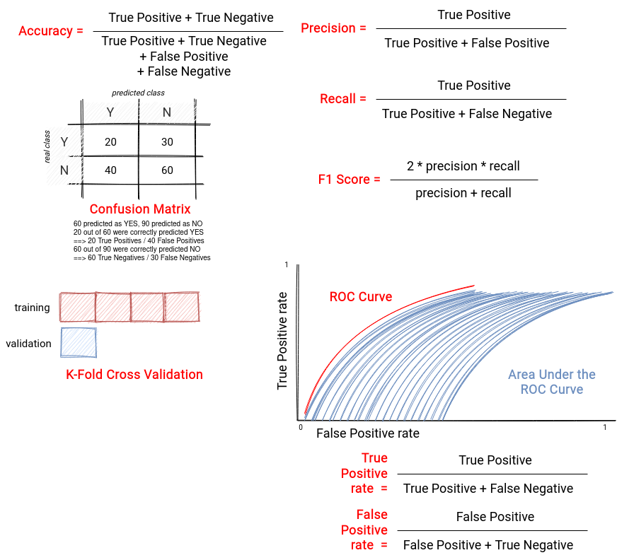
To decide whether the trained model can be deployed, we need to evaluate it and use one of the available metrics to estimate its quality. In the listing below you can find a summary for available evaluation methods:
- accuracy - probably the simplest method from the list since it defines the proportion of correctly predicted items. Doesn't perform good for unbalanced datasets (classification).
- precision - defines the proportion of real true positives among all positive cases identified (true positives and false positives; i.e. the cases identified as positives that in fact are negatives). In other words, this measure says how often the prediction will be correct. Good to use when most of the output are the positives.
- recall - measures the number of correctly identified positives. It's the opposite of precision, hence a good measure when most of the outputs are negatives.
- F1 Score - aka weighted average of precision and recall, more useful than accuracy if the dataset has an uneven class distribution.
- K-Fold Cross Validation - the evaluation process dividing the dataset into k groups. In every iteration, it keeps one group aside for evaluation. The remaining ones are used in training.
- confusion matrix - a matrix used in classification models helping to visually identify correctly and incorrectly classified values.
- ROC curve - a visual representation of the classification model performance at all classification thresholds. How to interpret it? The curves closer to 1 in the y axis are better, so the ones that are visually "higher" represent better models. The curve can be completed with Area Under the ROC Curve which can be interpreted as a probability of classifying a randomly chosen positive example higher than a randomly chosen negative example. If equal to 0.5, it means that the prediction is as good as random.
And the same listing but as an image:
For other ML problems like regression, you can use the measures like Root Mean Squared Error (good for a lot of data points and no outliers), Mean Squared Error (good if outliers have to be penalized), Mean Absolute Error (doesn't give the information if the model overfits or underfits).
Overfitting, underfitting
Model evaluation also helps to detect whether the model overfits or underfits. Underfitting, which is the first of 2 performance terms, occurs when the model can't learn from the data. In more format terms, we say that it can't accurately capture the relationship between the features and target variables.
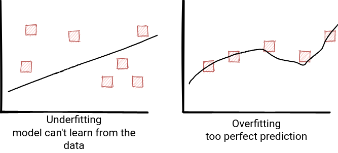
On the opposite side you will find the overfitting. When the model overfits, it often means that it remembers the training data instead of learning from it. It cannot be then generalized and applied to the unseen input. But fortunately, you can do something to improve the situation:
- underfitting, if occurs, it may be due to the model simplicity. Therefore, to fix it, we could start by complexifying it, like adding new features. If it doesn't work, you can try to use a different algorithm, add more training data, or fine-tune hyperparameters.
- overfitting can happen because of the model complexity or the training dataset issues. To fix the "model complexity" point you can use regularization. In simple terms, it consists of penalizing weights. To recall, a weight defines how a given feature is important in the model. 0 means here that the feature doesn't have any impact on the model. Without entering too much into details, there are 2 regularization levels called L1 and L2 and the difference is that the L1 can reduce the weight to 0 and eliminate it from the model.
Regularization also exists for neural networks and is called dropout regularization. The idea is to remove a random selection of a fixed number of units in a network layer.
But overfitting can also happen because of an inappropriate training dataset. Suppose it contains the features representing only one specific observation, and during the serving stage, you get the features representing a different observation. In that case, the model cannot be trained efficiently. To fix that, nothing complicated, include the unseen points to the training dataset.
Serving
Once trained and evaluated, the model can be finally served. What's interesting for data engineers is how to query it in batch and streaming processing. And more exactly, what are the best practices for that. GCP's recommended approach for batch processing is to use direct-model approach; i.e., downloading the model directly to the data processing pipeline. It can be further optimized with the creation of micro-batches passed to the prediction method.
For streaming pipelines, direct-model is also a recommended approach. Once again, the pipeline downloads the model and uses it locally for prediction. But there is a problem too. Streaming processing is supposed to run forever, and during the whole lifecycle, data scientists can deploy new versions of the model. The pipeline has to detect or be notified about that. And if it's something you cannot afford, it means that you have to use online approach; i.e., query the HTTP endpoint exposing the model. Here too, you can use micro-batch to improve the throughput but sending one request for multiple input parameters.
I'm pretty sure that you knew a lot of the things presented here. At the same time, I hope that you also learned something new, like me. Before preparing this article, I didn't know that TPU could be cheaper for some workloads or that we could use micro-batch for prediction! I was also very often confused about the model evaluation measures but having the visual support from this article helped my learning process. And you, there is something useful you discovered here?
Data Engineering Design Patterns

Looking for a book that defines and solves most common data engineering problems? I wrote
one on that topic! You can read it online
on the O'Reilly platform,
or get a print copy on Amazon.
I also help solve your data engineering problems contact@waitingforcode.com 📩
Read also about ML for data engineers - what I learned when preparing GCP Data Engineer certification here:
- Data preprocessing for machine learning: options and recommendations Data preprocessing for machine learning using TensorFlow Transform Machine Learning with Structured Data: Training the Model (Part 2) Comparing Machine Learning Models for Predictions in Cloud Dataflow Pipelines How to Use ROC Curves and Precision-Recall Curves for Classification in Python Classification: ROC Curve and AUC
Related blog posts:
- On tests in data systems
- Alerts, guards, and data engineering
- Agnostic data alerts with ydata-profiling
ML concepts were one of the hardest things to understand in my #GCP Data Engineer exam preparation. To help myself I wrote a blog post explaining the various concepts I discovered ? https://t.co/N9qjnIpaPA
— Bartosz Konieczny (@waitingforcode) March 28, 2021