
Using the right tool at the right time is important in every domain. It's particularly useful in the case of collections that can have different complexity for writing and reading. And very often this difference can dictate the use of one specific implementation.
What would it take for you to trust your Databricks pipelines in production?
A 3-day bug hunt on a 3-person team costs up to €7,200 in lost engineering time. This workshop teaches you to prevent that — unit tests, data tests, and integration tests for PySpark and Databricks Lakeflow, including Spark Declarative Pipelines.

Konieczny
This post is the first post from the series explaining the complexity of Scala collections. It shows the immutable collections. The post is organized differently than usual (no learning tests). Each collection is shortly presented in separate section and only at the end the complexities of all of them are shown in comparison table.
List
The List is a finite sequence of ordered not indexed elements. It performs pretty well for operations on head and tail of the sequence (O(1)) but has some troubles in random access patterns, e.g. index-basis. To find the item at specified index, it has to iterate over all items, up to specified index. For instance, if we need to access the 100th element, we'll need to traverse the first 99th entries before reaching the looked one.
The list also has different performance on writing. Adding the element at the beginning of the list (append) is made in constant time (O(1)). But doing the same but for the end of the list is done in linear time (O(n)). Why this difference ? A list is the data structure composed of one-way linked cons cells. It's terminated by a con cell called Nil. Once constructed it looks as in the following image:
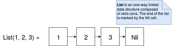
Prepending an element to already created immutable list simply adds new con cells at the beginning and links it to the first entry of existent list. But appending new item violates the immutability because we need to overwrite the link between the 3 and Nil elements in our case. It's why the solution for this problem is to duplicate the elements from the list to a new structure with the appended element at the end.
Stream
Stream is similar to List, except some subtle differences. The first one is that stream is computed lazily, item per item, only when it's requested. Once computed, the value remains in the sequence and can be reused without recomputation. The other difference are the boundaries. List is bounded while the stream is not.
But the laziness can be often a trap. Reading all elements, even in lazy manner, doesn't prevent against OOM problems. The sensible operations from this aspect are: size, max, sum and of course transformation methods, as toList.
Because of similarities with List, the complexity for all operations resumed in the table at the end, is the same as in the case of List.
Vector
A solution for poor performances of random accesses and prepend operations of list and streams is Vector. This data structure is a tree with high branching (32) factor composed of 6 layers of arrays. Thanks to that we can reach the first 32 elements directly (= the 1st branch has the size of 32), 1024 (32*32) elements with 1 level of indirection (= the 2nd branch has the size of 32^2), 32768 (32*32*32) with 2 levels of indirection (= the 3rd branch has the size of 32^3) and so on. Because of these indirection levels vector's complexity is expressed in effective constant time. It's effective because, for instance for reading, it has to get one element from each level's array (per index, so O(1) complexity).
Vectors are immutable but they support update operation (updated(index: Int, elem: B) method). The update will copy the node containing the updated element and every node that points to it. It creates 1-5 nodes (because of up to 6 array layers), each having 32 elements or subtrees. It's much slower than in-place replacement but it's cheaper than copying all values. So it's also done within effective constant time too.
Queue
Scala's Queue is a FIFO sequence. An interesting thing is the implementation. Internally the immutable queue is represented as 2 lists: the first for enqueuing and the second for dequeuing values:
sealed class Queue[+A] protected(protected val in: List[A], protected val out: List[A]) {
  def enqueue[B >: A](elem: B) = new Queue(elem :: in, out)

  def dequeue: (A, Queue[A]) = out match {
    case Nil if !in.isEmpty => val rev = in.reverse ; (rev.head, new Queue(Nil, rev.tail))
    case x :: xs            => (x, new Queue(in, xs))
    case _                  => throw new NoSuchElementException("dequeue on empty queue")
  }

}
The enqueue and dequeue operations execution flow is shown in the images below:
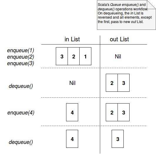
As you can see, the add operation is constant time because of previously explained constant time execution for List's append operation. But for dequeue, the complexity is amortized constant time. It's amortized because sometimes the usual head operation is replaced by the reversing the order of elements in the in List and moving it to the out part. But this reverse operation is supposed to happen from time to time, hence it's "amortized". You can learn a little bit more about already mentioned effective and amortized contant times in the post about Amortized and effective constant time complexities.
Range
Range is a sequence of equally spaced integers. It means that "3, 6, 9" is a range but "3, 6, 12, 24" is not. Internally it's composed of 3 elements: the start number, the end number and the stepping value. The stepping value determines the next returned number.
It's pretty efficient (constant time execution time) for the operations returning the first, the last and any random element of the range. The random access is a simple computation based on starting value, stepping value and requested index:
// implementation from Scala 2.12.1
final def apply(idx: Int): Int = {
  validateMaxLength()
  if (idx < 0 || idx >= numRangeElements) throw new IndexOutOfBoundsException(idx.toString)
  else start + (step * idx)
}
String
Some people ingore this fact but String is also an immutable collection. Internally it's implemented as an array of chars. Thanks to that it inherits good random access results (constant time, since chars array is queried).
But writing operations performs in linear time. It's because of copying the chars array into new string object. It's for instance the case of concatenation operation that in terms of Scala's comparison table can be considered as append or prepend operation:
public String concat(String str) {
    int otherLen = str.length();
    if (otherLen == 0) {
        return this;
    }
    int len = value.length;
    char buf[] = Arrays.copyOf(value, len + otherLen);
    str.getChars(buf, len);
    return new String(buf, true);
}
Also the updating (replace in String) occurs in linear time:
public String replace(char oldChar, char newChar) {
  if (oldChar != newChar) {
    int len = value.length;
    int i = -1;
    char[] val = value; /* avoid getfield opcode */

    while (++i < len) {
      if (val[i] == oldChar) {
        break;
      }
    }
    if (i < len) {
      char buf[] = new char[len];
      for (int j = 0; j < i; j++) {
        buf[j] = val[j];
      }
      while (i < len) {
        char c = val[i];
        buf[i] = (c == oldChar) ? newChar : c;
        i++;
      }
      return new String(buf, true);
    }
  }
  return this;
}
Complexity comparison table
After describing some main immutable sequences (Stack omitted because it's marked as deprecated), it's time to resume their complexities in the table below (same as Collections Performance Characteristics but in Big O notation):
| collection | head | tail | access per index | update | prepend | append |
|---|---|---|---|---|---|---|
| List | O(1) | O(1) | O(n) | O(n) | O(1) | O(n) |
| Stream | O(1) | O(1) | O(n) | O(n) | O(1) | O(n) |
| Vector | e.O(1) | e.O(1) | e.O(1) | e.O(1) | e.O(1) | e.O(1) |
| Queue | a.O(1) | a.O(1) | O(n) | O(n) | O(1) | O(1) |
| Range | O(1) | O(1) | O(1) | - | - | - |
| String | O(1) | O(n) | O(1) | O(n) | O(n) | O(n) |
e.O(1) is the abbreviation used for effective constant time and a.O(1) for amortized constant time.
This post explains the time complexity of main immutable Scala's sequences. It's composed of 7 parts. The first 6 parts show some implementation details of: List, Stream, Vector, Queue, Range and String types. Each of them helps to understand why some operations take more time than the others in terms of complexity. We can often see that it depends on constructions used to store the data. The last part resumes the complexities in a single table those is good to have close at hand every time when we deal with a collection composed of a lot of entries.
Data Engineering Design Patterns

Looking for a book that defines and solves most common data engineering problems? I wrote
one on that topic! You can read it online
on the O'Reilly platform,
or get a print copy on Amazon.
I also help solve your data engineering problems contact@waitingforcode.com 📩
Read also about Collections complexity in Scala - immutable collections here:
- Why exactly is prepend to a Scala List a constant time operation, but append a linear time operation? Concrete Immutable Collection Classes Immutable data structures
Related blog posts:
- The day I was punished by the mutability
- Stream safely in Scala
- Scala mutable collections
- Amortized and effective constant time
The 1st post about #Scala and its immutable collections complexity https://t.co/yirmJ5H3dD pic.twitter.com/qhniciu4G9
— bardev (@waitingforcode) October 1, 2017