
I wanted to write this post after the one about aggregation modes but I didn't. Before explaining different aggregation strategies, I prefer to clarify aggregation internals. It should help you to better understand the next part.
What would it take for you to trust your Databricks pipelines in production?
A 3-day bug hunt on a 3-person team costs up to €7,200 in lost engineering time. This workshop teaches you to prevent that — unit tests, data tests, and integration tests for PySpark and Databricks Lakeflow, including Spark Declarative Pipelines.

Konieczny
The post is composed of 4 sections. In the first one, I will introduce the main classes involved in the aggregations creation. In the 2 next sections, I will cover the creation of physical plans for the aggregation with and without the distinct operator. In the last part, I will discuss 3 different execution strategies for aggregates.
Aggregation construction
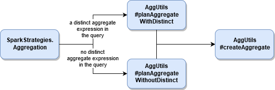
An important part in construction of the aggregation query is org.apache.spark.sql.execution.aggregate.AggUtils. It exposes 3 methods that are called by org.apache.spark.sql.execution.SparkStrategies.Aggregation and org.apache.spark.sql.execution.SparkStrategies.StatefulAggregationStrategy execution strategies. These 3 methods transform the specified aggregations into the physical plan and they're all doing that by invoking this private method:
  private def createAggregate(
      requiredChildDistributionExpressions: Option[Seq[Expression]] = None,
      groupingExpressions: Seq[NamedExpression] = Nil,
      aggregateExpressions: Seq[AggregateExpression] = Nil,
      aggregateAttributes: Seq[Attribute] = Nil,
      initialInputBufferOffset: Int = 0,
      resultExpressions: Seq[NamedExpression] = Nil,
      child: SparkPlan): SparkPlan
In this post I'll omit the stateful aggregation and try to describe it in a dedicated post.
Distinct aggregation algorithm
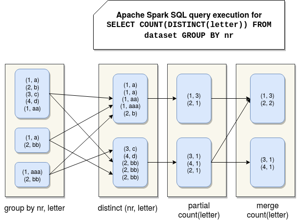
The aggregation with a distinct clause is composed of 4 physical execution nodes. I will analyze them for the following query:
val dataset = Seq(
(1, "a"), (1, "a"), (1, "a"), (2, "b"), (2, "b"), (3, "c"), (3, "c")
).toDF("nr", "letter")

dataset.groupBy($"nr").agg(functions.countDistinct("letter")).explain(true)
- partial aggregation node - this first stage creates a partial aggregate for the distinct aggregation. This partial aggregation won't use the grouping key from the query but the keys defining the unicity of rows in the query. It means that instead of grouping by "nr" column, it will group by "nr" and "letter" columns, and you can see that pretty well in the corresponding part of the execution plan:
HashAggregate(keys=[nr#5, letter#6], functions=[], output=[nr#5, letter#6])
  +- LocalTableScan [nr#5, letter#6]
- partial merge aggregation node - the execution plan is identical to the plan from the previous point. The difference is that this operation happens after the shuffle, so after moving all rows with the same (nr, letter) keys on the same partition:
+- HashAggregate(keys=[nr#5, letter#6], functions=[], output=[nr#5, letter#6])
   +- Exchange hashpartitioning(nr#5, letter#6, 200)
        +- HashAggregate(keys=[nr#5, letter#6], functions=[], output=[nr#5, letter#6])
            +- LocalTableScan [nr#5, letter#6]
At this moment Apache Spark guaranteed the distinct character of our query. And directly from that it can move on. - partial aggregation for distinct node - during this stage Spark finally starts to execute the aggregation. The execution is partial and you can notice that by analyzing the execution plan:
+- HashAggregate(keys=[nr#5], functions=[partial_count(distinct letter#6)], output=[nr#5, count#18L]) +- HashAggregate(keys=[nr#5, letter#6], functions=[], output=[nr#5, letter#6]) +- Exchange hashpartitioning(nr#5, letter#6, 200) +- HashAggregate(keys=[nr#5, letter#6], functions=[], output=[nr#5, letter#6]) +- LocalTableScan [nr#5, letter#6] - final aggregation - it's here where partially aggregated results are merged into the final result and are returned to the client's program. It involves shuffling the data:
HashAggregate(keys=[nr#5], functions=[count(distinct letter#6)], output=[nr#5, count(DISTINCT letter)#12L])
+- Exchange hashpartitioning(nr#5, 200)
      +- HashAggregate(keys=[nr#5], functions=[partial_count(distinct letter#6)], output=[nr#5, count#18L])
             +- HashAggregate(keys=[nr#5, letter#6], functions=[], output=[nr#5, letter#6])
                +- Exchange hashpartitioning(nr#5, letter#6, 200)
                   +- HashAggregate(keys=[nr#5, letter#6], functions=[], output=[nr#5, letter#6])
                      +- LocalTableScan [nr#5, letter#6]
And a picture to summarize these steps:
No distinct aggregation algorithm
The execution plan for an aggregation without distinct operator is much simpler since it consists of only 2 nodes. I'll analyze it for this example:
val dataset = Seq(
  (1, "a"), (1, "a"), (1, "a"), (2, "b"), (2, "b"), (3, "c"), (3, "c")
).toDF("nr", "letter")
dataset.groupBy($"nr").count().explain(true)
- partial aggregations node - the first step corresponds to the partial aggregation:
HashAggregate(keys=[nr#5], functions=[partial_count(1)], output=[nr#5, count#17L])
+- PlanLater LocalRelation [nr#5]
- final aggregation node - and no mystery here, the final aggregation of the partial results are made:
HashAggregate(keys=[nr#5], functions=[count(1)], output=[nr#5, count#12L])
+- HashAggregate(keys=[nr#5], functions=[partial_count(1)], output=[nr#5, count#17L])
   +- PlanLater LocalRelation [nr#5]
Hash-based vs sort-based aggregation
When any of 2 previously presented aggregation modes is executed, it goes to a method called createAggregate. This function creates a physical node corresponding to the one of 3 aggregation strategies, hash-based, object-hash-based and sort-based. I will cover them in this section. But before, I'll introduce some common concepts.
An Apache Spark SQL's aggregation is mainly composed of 2 parts, an aggregation buffer, and an aggregation state. Every time when you call GROUP BY key and use some aggregations on them, the framework creates an aggregation buffer which is reserved to the given aggregation (GROUP BY key). Any aggregation involved for given key (COUNT, SUM,...) stores there its partial aggregation result called aggregation state. The storage format of that state depends on the aggregation. For AVG it will be 2 cells, one for the number of occurrences and another for the sum of the values, for MIN it will be the minimum value seen so far and so forth. Soon you will understand why it's important.
The first strategy, hash-based uses mutable and primitive types with fixed sizes as aggregate states, so for instance longs, doubles, dates, timestamps, floats, booleans, ... - you'll find the full list in UnsafeRow#isMutable(DataType dt) method. The mutability is so important here because Apache Spark will change the values of the aggregation in the buffer directly in place. For any other type the object-hash-based strategy is used. It was introduced in the release 2.2.0 in order to address the limitations of the hash-based strategy. Prior 2.2.0 any aggregation executed against other types that the ones supported by HashAggregateExec, was transformed to the sort-based strategy. However, most of the time SortAggregateExec will be less efficient than its hash-based alternative since it involves extra sorting steps before making the aggregation. Starting from 2.2.0, if the configuration doesn't say the opposite, object-hash based approach will be preferred over the sort-based. And the configuration property controlling that behavior is spark.sql.execution.useObjectHashAggregateExec, set to true by default. To understand the difference between hash and sort aggregations, you can compare these 2 plans below for that query:
val dataset2 = Seq(
      (1, "a"), (1, "aa"), (1, "a"), (2, "b"), (2, "b"), (3, "c"), (3, "c")
    ).toDF("nr", "letter")
    dataset2.groupBy("nr").agg(functions.collect_list("letter").as("collected_letters")).explain(true)
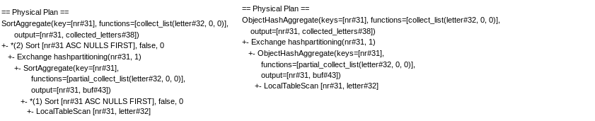
As you can see, in both cases the data is shuffled only once but for the sort-based execution, the data must be sorted twice which can introduce an important overhead regarding the hash execution.
Another interesting thing to notice is that both hash-based aggregates can fallback into sort-based aggregation in case of any memory problems detected at runtime. For object hash-based aggregation it's controlled by the number of keys in the map configured with spark.sql.objectHashAggregate.sortBased.fallbackThreshold property. By default, this value is set to 128 so it means that you will only be able to store the aggregates for 128 keys. In case of fallback, you will see the messages like:
ObjectAggregationIterator: Aggregation hash map reaches threshold capacity (128 entries), spilling and falling back to sort based aggregation. You may change the threshold by adjust option spark.sql.objectHashAggregate.sortBased.fallbackThreshold
For hash-based execution, the fallback is controlled by BytesToBytesMap class and its max capacity configuration which is of 2^29 keys.
In this post I wanted to show you some basics about the execution of aggregations in Apache Spark SQL. The first part introduced the AggUtils which is the object responsible for the creation of physical plans. The physical plans which were covered in the next 2 sections. As we could all expect, the plan for the query without the distinct operation is much simpler. Both query execution plans have things in common though like partial aggregation. I'll explain that topic more in the next post from the series. Finally, in the last part, you could learn about 3 different execution strategies. 2 of them are hash-based and use a hash map where the aggregation results are stored. The last one, and at the same time the less efficient, is sort-based and involves extra sorting steps in the physical plan.
Data Engineering Design Patterns

Looking for a book that defines and solves most common data engineering problems? I wrote
one on that topic! You can read it online
on the O'Reilly platform,
or get a print copy on Amazon.
I also help solve your data engineering problems contact@waitingforcode.com 📩
Read also about Aggregations execution in Apache Spark SQL here:
Related blog posts:
Some time ago, I was analyzing the query plan generated by my #ApacheSpark app and found a mysterious partial operations. I decided then to investigate and today's post starts a series about aggregations in #SparkSQL https://t.co/4VgaFJqxK5
— Bartosz Konieczny (@waitingforcode) October 12, 2019