
In my previous post I explained how Apache Spark can reorder JOINs based on the logical plan. Today I'll focus on another aspect of reordering which uses cost estimation for the proposed plans.
What would it take for you to trust your Databricks pipelines in production?
A 3-day bug hunt on a 3-person team costs up to €7,200 in lost engineering time. This workshop teaches you to prevent that — unit tests, data tests, and integration tests for PySpark and Databricks Lakeflow, including Spark Declarative Pipelines.

Konieczny
I've already covered cost-based part of Apache Spark by the past in Spark SQL Cost-Based Optimizer post so here I will really focus only on the part related to the JOIN operation. And I will start with a short section on the high level view of this optimization. In the next one I will present the algorithm used to figure out the most effective query plan. Before terminating this article, I will show some code snippets proving the optimization.
Reordering joins - the cost-based version
Cost-based reorder join uses cost related to the query and that's the reason why its execution is conditioned. it's chosen when all of the following requirements are met:
- CBO properties enabled - spark.sql.cbo.enabled and spark.sql.cbo.joinReorder.enabled, both by default set to false, must be enabled.
- a join condition exists - so if you execute SELECT t1.*,t2.*, t3.* FROM table1 AS t1, table2 AS t2, table3 AS t3, the optimization won't apply
- at least 3 and at most spark.sql.cbo.joinReorder.dp.threshold join tables are used - so it won't work for a query like SELECT t1.*,t2.* FROM table1 AS t1, table2 AS t2 WHERE t1.id = t2.id
- all join tables must have statistics updated with the estimated number of rows
Dynamic programming reordering
The execution flow starts with a standard pattern matching on the query plan nodes. If one of them matches, the reorder(plan: LogicalPlan, output: Seq[Attribute]) method from CostBasedReorderJoin's is invoked. Inside this method, Apache Spark first retrieves all tables and conditions involved in the query. If the reorder join can be applied (cf: see the list with 4 bullet points from the previous section), the framework transforms the initial plan with the help of a dynamic programming algorithm from JoinReorderDP class. As for any dynamic programming algorithm, the idea here is to divide one big problem into smaller ones and use their results to solve the overall problem.
From a high-level view, the algorithm starts by decomposing the plan into 2 main components: sources and join conditions. Later it starts by initializing the first level of the possible plans by putting all sources at the same level like [(source1), (source2), (source3)]. Such prepared input is later passed to searchLevel(existingLevels: Seq[JoinPlanMap],conf: SQLConf, conditions: Set[Expression], topOutput: AttributeSet, filters: Option[JoinGraphInfo]) method which is responsible for the generation of the next level's combination. Inside, the algorithm tries to figure out the most optimal join structure by testing all possible join combinations at every level. So for the first execution, it will compare the joins between source1 - source2, source1 - source3 and source2 - source3.
You may think now that illogical joins will be generated but that won't happen. Join candidates are passed to a method called buildJoin. It returns None if both query sides cannot be joined. The "joinability" is conditioned by the overlapping (both sides are different) and at least one join condition applicable to both sides:
// ...
    if (oneJoinPlan.itemIds.intersect(otherJoinPlan.itemIds).nonEmpty) {
      // Should not join two overlapping item sets.
      return None
    }
// ...
    val onePlan = oneJoinPlan.plan
    val otherPlan = otherJoinPlan.plan
    val joinConds = conditions
      .filterNot(l => canEvaluate(l, onePlan))
      .filterNot(r => canEvaluate(r, otherPlan))
      .filter(e => e.references.subsetOf(onePlan.outputSet ++ otherPlan.outputSet))
    if (joinConds.isEmpty) {
      // Cartesian product is very expensive, so we exclude them from candidate plans.
      // This also significantly reduces the search space.
      return None
    }
When both sides can be joined, the algorithm estimates their cost and updates the logical plan stored for a specific combination of tables (items in the snippet):
    val nextLevel = mutable.Map.empty[Set[Int], JoinPlan]

              // Check if it's the first plan for the item set, or it's a better plan than
              // the existing one due to lower cost.
              val existingPlan = nextLevel.get(newJoinPlan.itemIds)
              if (existingPlan.isEmpty || newJoinPlan.betterThan(existingPlan.get, conf)) {
                nextLevel.update(newJoinPlan.itemIds, newJoinPlan)
              }

    def betterThan(other: JoinPlan, conf: SQLConf): Boolean = {
      if (other.planCost.card == 0 || other.planCost.size == 0) {
        false
      } else {
        val relativeRows = BigDecimal(this.planCost.card) / BigDecimal(other.planCost.card)
        val relativeSize = BigDecimal(this.planCost.size) / BigDecimal(other.planCost.size)
        relativeRows * conf.joinReorderCardWeight +
          relativeSize * (1 - conf.joinReorderCardWeight) < 1
      }
    }
The cost formula is rows * weight + size * (1 - weight) where the weight is defined as spark.sql.cbo.joinReorder.card.weight property.
At every level the algorithm will keep only the best plan for each combination of items and at the end compose the final plan from them. Every iteration doesn't take all prior plans. The part of the algorithm responsible for selecting the plans computed previously looks like:
var k = 0
val lev = existingLevels.length - 1
while (k <= lev - k) {
   // take plans for k level
   k += 1
}
As you can see, for the level 3, only the first 2 levels will be used.
Dynamic programming reordering illustrated
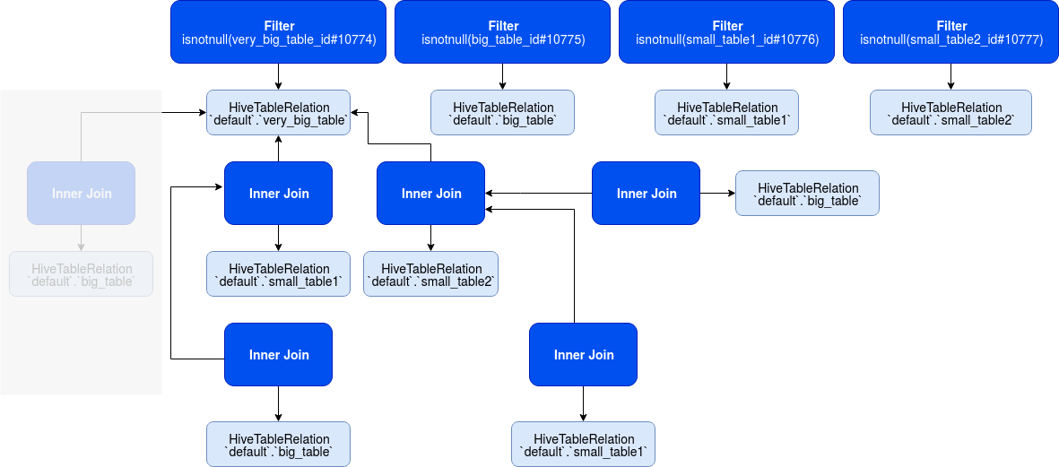
Even though I pointed out some methods involved in this algorithm, I beat that it's still a little bit mysterious. To understand the idea better, let's imagine 4 tables, a very big one (5000 rows), a big one (1500 rows) and 2 small ones (respectively 800 and 200 rows). We want to join them that way:
SELECT vb.*, b.*, s1.*, s2.*
FROM very_big_table AS vb
JOIN big_table AS  b ON vb.very_big_table_id = b.big_table_id
JOIN small_table1 AS s1 ON vb.very_big_table_id = s1.small_table1_id
JOIN small_table2 AS s2 ON vb.very_big_table_id = s2.small_table2_id
For the sake of simplicity, I will use table aliases in the rest of this part, so vb will stand for very_big_table, b for big_table and so on.
Below you can find the final result of the transformation without the intermediary steps that I will detail just after:
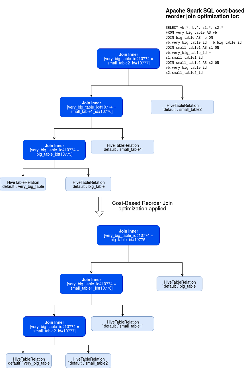
As you can see, in the analyzed query, Apache Spark starts by joining the 2 biggest tables whereas, in its optimized version, it does the opposite and joins the smallest tables first. It can be explained by the dynamic programming algorithm executed in these steps:
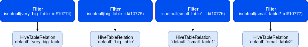
1. Setup
In this initial stage, the algorithm retrieves all tables involved in the join as well as the conditions used in the joins. It also tries to find star schema patterns but for the sake of simplicity, I will present star schema optimization in one of the next articles. Four our test query, the setup will produce 4 tables, 3 conditions and the starting (0) level of combinations:
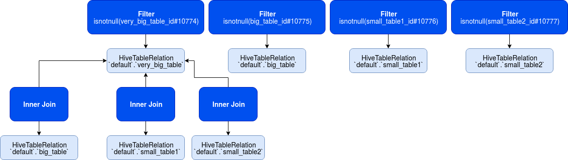
2. Level 1 generation
In the next step, the algorithm retrieves the most optimal join for every table involved in the query. It's doing that by combining every single item with another and checking whether the join can be made and if yes, whether it's cheaper than the current join. The iteration tries these pairs: (vb, vb), (vb, b), (vb, s1), (vb, s2), (b, b), (b, s1), (b, s2), (s1, s1), (s1, s2), (s2, s2).
As you can see, the combinations already tested like (vb, b) are omitted for the subsequent items. This behavior is controlled here (see "Both sides of ..." comment):
    while (k <= lev - k) {
      val oneSideCandidates = existingLevels(k).values.toSeq
      for (i <- oneSideCandidates.indices) {
        val oneSidePlan = oneSideCandidates(i)
        val otherSideCandidates = if (k == lev - k) {
          // Both sides of a join are at the same level, no need to repeat for previous ones.
          oneSideCandidates.drop(i)
        } else {
          existingLevels(lev - k).values.toSeq
        }
Invalid pairs are of course skipped. The result of this step looks like that:
2. Level 2 generation
The 2nd level generation takes all results from the previous step and combines them, still by keeping the cheapest option as the output. In other words, the algorithm combines all basic joins and figures out the cheapest combinations. In the following picture, you can see some of the combined plans at this stage alongside their costs:
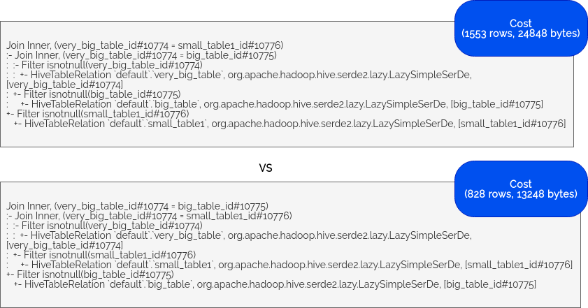
The outcome of this level looks like:
As you can see, the algorithm created new pairs between (b, (vb, s2)), (b, (vb, s1)), (s1, (vb, s2)).
2. Level 3 generation
That's the final step which starts by comparing the values from the setup stage [(vb), (b), (s1), (s2)] with the pairs generated before. It happens because of the else side:
        val oneSidePlan = oneSideCandidates(i)
        val otherSideCandidates = if (k == lev - k) {
          // Both sides of a join are at the same level, no need to repeat for previous ones.
          oneSideCandidates.drop(i)
        } else {
          existingLevels(lev - k).values.toSeq
        }
This first execution of this level generates the following combinations: [vb, (s1, vb, s2)], [vb, (b, vb, s1)], [vb, (b, vb, s2)], [b, (s1, vb, s2)], [b, (b, vb, s1)], [b, (b, vb, s2)], [s1, (s1, vb, s2)], [s1, (b, vb, s1)], [s1, (b, vb, s2)], [s2, (s1, vb, s2)], [s2, (b, vb, s1)], [s2, (b, vb, s2)]. I highlighted here the final plan but the algorithm executes also another step where it compares the pairs generated in the level 1. However, none of the combinations is adequate since this execution works on oneSideCandidates and generates [(vb, s2), (vb, s2)], [(vb, s2), (vb, b)], [(vb, s2), (vb, s1)], [(vb, b), (vb, b)], [(vb, b), (vb, s1)], [(vb, s1), (vb, s1)]. All these pairs are rejected because of working on overlapping items. Below you can find the condition from buildJoin method responsible for rejecting all of these pairs:
    if (oneJoinPlan.itemIds.intersect(otherJoinPlan.itemIds).nonEmpty) {
      // Should not join two overlapping item sets.
      return None
    }
At the end, the chosen plan is first transformed to an intermediary node represented by OrderedJoin class which, before leaving the optimization logic, is transformed back to Join node:
      // s
      result transformDown {
        case OrderedJoin(left, right, jt, cond) => Join(left, right, jt, cond)
      }
Why this intermediary format? I found the answer in Fix recursive join reordering: inside joins are not reordered ticket where the purpose of OrderedJoin is defined as:
In join reorder, we use `OrderedJoin` to indicate a join has been ordered, such that when transforming down the plan, these joins don't need to be reordered again.
Cost-based reorder join examples
Before terminate, let's see some code. In this part I took the example explained before, ie. 4 tables, 1 very big, 1 big and 2 small. Before executing the joins, I compute the statistics to give a little bit more context about the tables to the optimizer. In the final assertion, you can see that the CostBasedReorderJoin logical rule was applied. I won't recall here the transformed plan since it's the same as in the previous part:
FOR COLUMNS or not FOR COLUMNS?
In the snippet I use column-based statistics (FOR COLUMNS ${id}). That's because they give a better accuracy for the optimization. Thanks to them, Apache Spark can better estimate the size of each table by taking the average size of the column directly from the data catalog. If column statistics aren't computed, the framework simply takes a default size for given column type. Despite that, CBO will work for both cases (with/without column stats).
  private val enabled = "true"
  private val sparkSession: SparkSession = SparkSession.builder()
    .appName("Reorder JOIN CBO test")
    .config("spark.sql.cbo.joinReorder.enabled", s"${enabled}")
    .config("spark.sql.cbo.enabled",s"${enabled}")
    .config("spark.sql.cbo.joinReorder.dp.star.filter", s"${enabled}")
    .config("spark.sql.statistics.histogram.enabled", s"${enabled}")
    .config("spark.sql.shuffle.partitions", "1")
    .enableHiveSupport()
    .master("local[*]").getOrCreate()

  private val baseDir = "/tmp/cbo_reorder_join/"

  override def beforeAll(): Unit = {
    if (!new File(baseDir).exists()) {
      val veryBigTable = "very_big_table"
      val bigTable = "big_table"
      val smallTable1 = "small_table1"
      val smallTable2 = "small_table2"
      val configs = Map(
        veryBigTable -> 5000,
        bigTable -> 1500,
        smallTable1 -> 800,
        smallTable2 -> 200
      )
      configs.foreach {
        case (key, maxRows) => {
          val data = (1 to maxRows).map(nr => nr).mkString("\n")
          val dataFile = new File(s"${baseDir}${key}")
          FileUtils.writeStringToFile(dataFile, data)
          val id = s"${key}_id"
          sparkSession.sql(s"DROP TABLE IF EXISTS ${key}")
          sparkSession.sql(s"CREATE TABLE ${key} (${id} INT) USING hive OPTIONS (fileFormat 'textfile', fieldDelim ',')")
          sparkSession.sql(s"LOAD DATA LOCAL INPATH '${dataFile.getAbsolutePath}' INTO TABLE ${key}")
          sparkSession.sql(s"ANALYZE TABLE ${key} COMPUTE STATISTICS FOR COLUMNS ${id}")
        }
      }
    }
  }

  "cost-based reorder join" should "apply to a not optimized query join" in {
    val logAppender = InMemoryLogAppender.createLogAppender(
      Seq("Applying Rule org.apache.spark.sql.catalyst.optimizer.CostBasedJoinReorder"))

    sparkSession.sql(
      """
        |SELECT vb.*, b.*, s1.*, s2.*
        |FROM very_big_table AS vb
        |JOIN big_table AS  b ON vb.very_big_table_id = b.big_table_id
        |JOIN small_table1 AS s1 ON vb.very_big_table_id = s1.small_table1_id
        |JOIN small_table2 AS s2 ON vb.very_big_table_id = s2.small_table2_id
      """.stripMargin).explain(true)

    logAppender.getMessagesText() should have size 1
    logAppender.getMessagesText()(0).trim should startWith("=== Applying Rule org.apache.spark.sql.catalyst.optimizer.CostBasedJoinReorder ===")
  }
Cost-based join reorder is a very powerful tool in Apache Spark logical optimizations arsenal. It uses real physical information about the data to propose the most optimal query execution time. Thanks to the dynamic programming algorithm based on the "Access Path Selection in a Relational Database Management System" paper, Spark can choose the best plan and override the analyzed plan with it.
Data Engineering Design Patterns

Looking for a book that defines and solves most common data engineering problems? I wrote
one on that topic! You can read it online
on the O'Reilly platform,
or get a print copy on Amazon.
I also help solve your data engineering problems contact@waitingforcode.com 📩
Read also about Reorder JOIN optimizer - cost-based optimization here:
Related blog posts:
- Reorder JOIN optimizer - star schema
- Reorder JOIN optimizer
- Spark SQL Cost-Based Optimizer
- Spark SQL operator optimizations - part 1
- Predicate pushdown in Spark SQL
The second part of my join reorder series in #ApacheSpark #SparkSQL is online. Today it's time to focus on its cost-based part ? https://t.co/Hu7ptUuA6P
— Bartosz Konieczny (@waitingforcode) February 22, 2020