Spark Declarative Pipelines internals

🏷️ Apache Spark 4.1.0 https://github.com/bartosz25/spark-...aming-declarative-pipelines/pyspark

Welcome back to our series on Spark Declarative Pipelines (SDP)! So far, we've tackled the fundamentals of building jobs and the logistics of operationalizing them in production. Now that your pipelines are running smoothly, it's time to pop the hood and see what's actually happening under the surface.

Step 1: graph creation

In previous blog posts, you learned about the high-level execution flow. This process begins with the spark-pipelines run command, which invokes the pipelines/cli.py file under the hood. The cli.py file interacts with the remote SparkSession via various Protobuf messages that either declare execution graph resources or trigger the execution. This initial execution step is summarized in the diagram below:

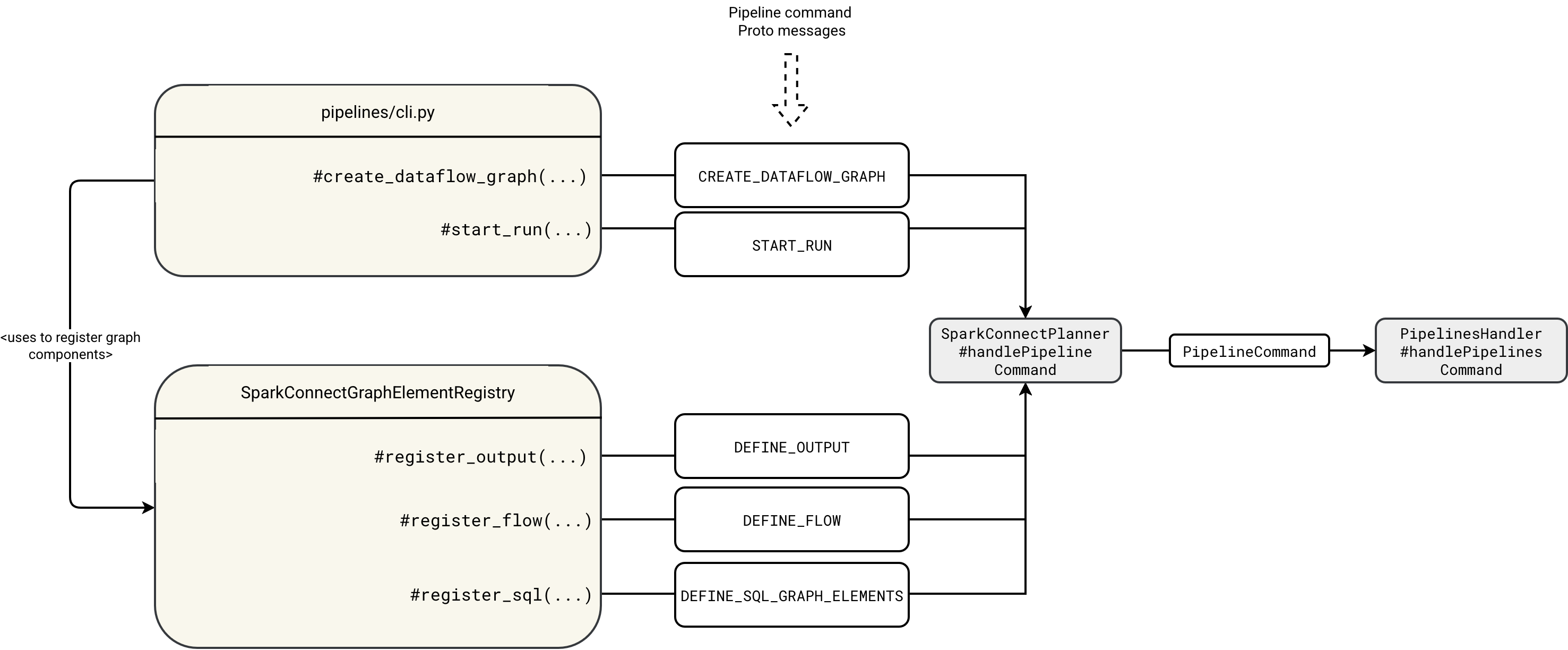
The workflow first starts by registering the empty graph in the DataflowGraphRegistry:

class DataflowGraphRegistry {

  private val dataflowGraphs = new ConcurrentHashMap[String, GraphRegistrationContext]()

  def createDataflowGraph(
      defaultCatalog: String, defaultDatabase: String, defaultSqlConf: Map[String, String]): String = {
    val graphId = java.util.UUID.randomUUID().toString
    dataflowGraphs.put(
      graphId, new GraphRegistrationContext(defaultCatalog, defaultDatabase, defaultSqlConf))
    graphId
  }

The cli.py reads the graph id and uses it to register the flows, outputs, and SQL scripts with appropriate DEFINE_ commands. Each flow, table or sink is later registered in the GraphRegistrationContext corresponding to the graph id:

class GraphRegistrationContext(
    val defaultCatalog: String,
    val defaultDatabase: String,
    val defaultSqlConf: Map[String, String]) {
  import GraphRegistrationContext._

  protected val tables = new mutable.ListBuffer[Table]
  protected val views = new mutable.ListBuffer[View]
  protected val sinks = new mutable.ListBuffer[Sink]
  protected val flows = new mutable.ListBuffer[UnresolvedFlow]

  def registerTable(tableDef: Table): Unit = tables += tableDef
  def registerView(viewDef: View): Unit = views += viewDef
  def registerSink(sinkDef: Sink): Unit = sinks += sinkDef

Step 2: execution

Once you register the complete graph, Apache Spark can proceed to the physical execution. It starts with the interception of the START_RUN command. The interception happens inside the PipelinesHandler that starts the workflow asynchronously. Because the execution is asynchronous, you can find an execution thread mentioned in the diagram illustrating the execution chain:

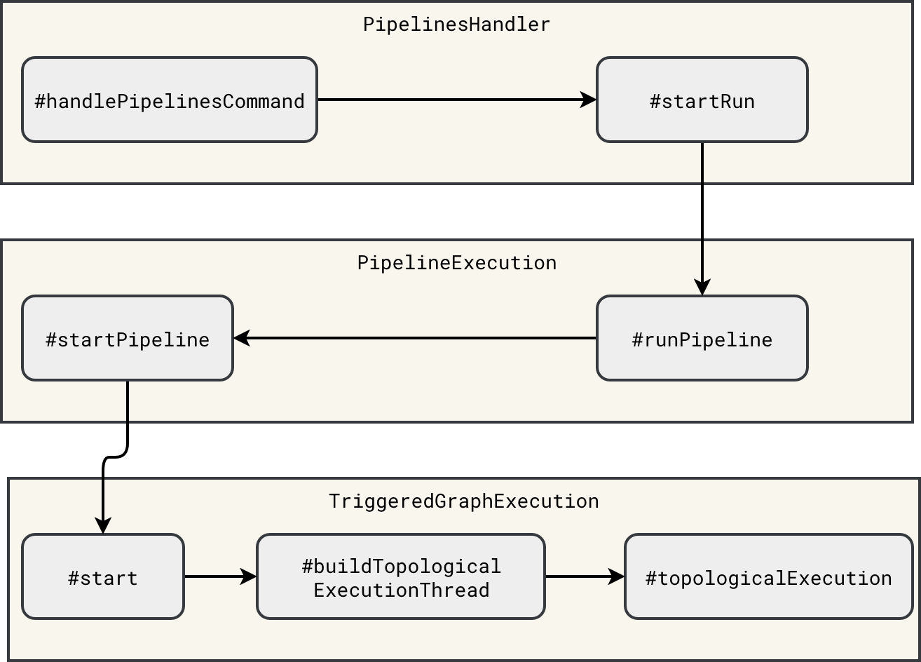
The execution thread starts in the TriggeredGraphExecution#start method:

override def start(): Unit = {
  // ...
  val thread = buildTopologicalExecutionThread()
  // ...
  thread.start()
    topologicalExecutionThread = Some(thread)
}

The execution itself is a two-steps process. The first step consists of translating the components of the DataflowGraph into runnable execution nodes - a little bit like with Apache Spark SQL execution plan where the query moves from the analyzed to logical, and finally, to physical forms. In SDP the physical planning is simplified as it consists of translating resolved logical nodes (Table, Sink) into their physical, hence runnable, components (BatchTableWrite, StreamingTableWrite, Sink). You can see this simplified planning step in the next diagram:

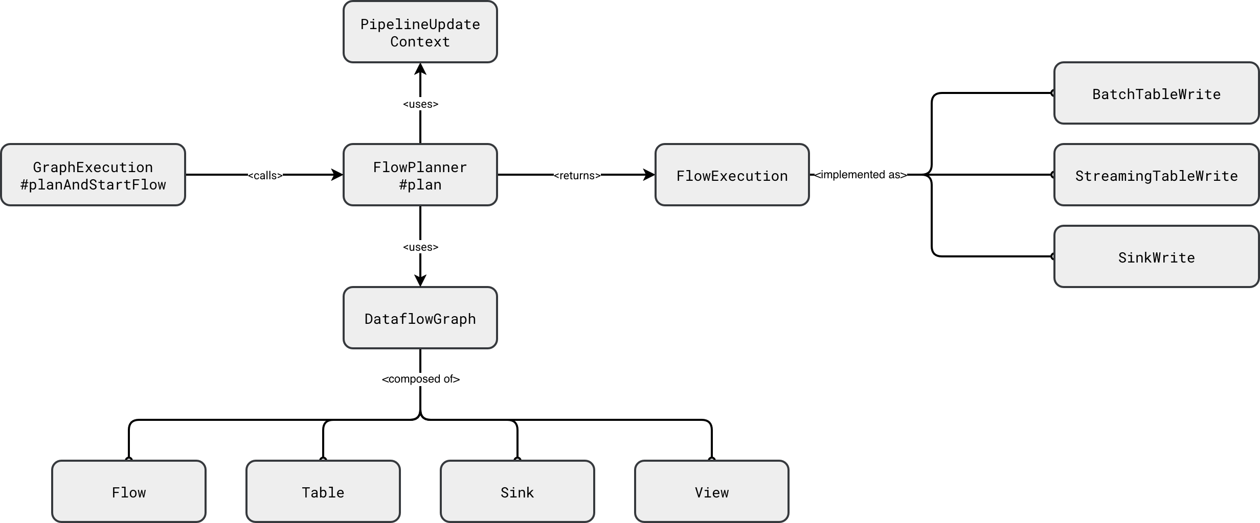
Under-the-hood all the FlowExecution physical nodes wrap the Apache Spark Structured Streaming code to execute a streaming query, or the Apache Spark SQL code to run a batch query:

class SinkWrite
  // ...
  def startStream(): StreamingQuery = {
    val data = graph.reanalyzeFlow(flow).df
    data.writeStream
      .queryName(displayName)
      .option("checkpointLocation", checkpointPath)
      .trigger(trigger)
      .outputMode(OutputMode.Append())
      .format(destination.format)
      .options(destination.options)
      .start()
  }
}

class StreamingTableWrite
  // ...
  def startStream(): StreamingQuery = {
    val data = graph.reanalyzeFlow(flow).df
    val dataStreamWriter = data
      .writeStream
      .queryName(displayName)
      .option("checkpointLocation", checkpointPath)
      .trigger(trigger)
      .outputMode(OutputMode.Append())
    destination.format.foreach(dataStreamWriter.format)
    dataStreamWriter.toTable(destination.identifier.unquotedString)
  }
}

class BatchTableWrite
  // ...
    def executeInternal(): Future[Unit] = {
    SparkSessionUtils.withSqlConf(spark, sqlConf.toList: _*) {
      // ...
      val data = graph.reanalyzeFlow(flow).df
      Future {
        val dataFrameWriter = data.write
        destination.format.foreach(dataFrameWriter.format)
        destination.clusterCols.foreach { clusterCols =>
          dataFrameWriter.clusterBy(clusterCols.head, clusterCols.tail: _*)
        }
        destination.partitionCols.foreach { partitionCols =>
          dataFrameWriter.partitionBy(partitionCols: _*)
        }
        dataFrameWriter
          .mode("append")
          .saveAsTable(destination.identifier.unquotedString)
      }
    }
  }
}

Caching, what caching?

After looking at the previous snippet you are certainly asking yourself, what if two sinks reference the same upstream flow. If you write this in Apache Spark Structured Streaming API as two separate streaming queries, you don't have a guarantee both queries will process the same data. If it's something new for you, I analyzed this part in 2023's blog post Multiple queries running in Apache Spark Structured Streaming.

The answer is - as usual - it depends. It depends on what the upstream node is. To illustrate it better, let's see how SDP planner creates physical DataFrames holding the processed datasets:

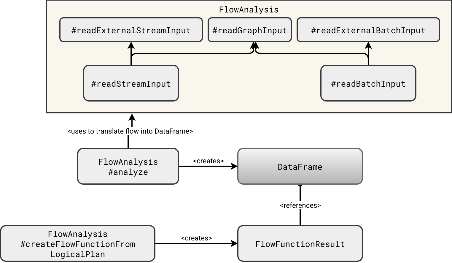
As you can see in the schema, the DataFrame is created from one of two functions. If the upstream dependency is created inside the SDP pipeline, then the planner uses the readGraphInput. Otherwise, it resovles the node by calling one of the readExternal...Input. The difference between these two? The graph input creates a DataFrame from the rows belonging to the upstream node which are kept in memory:

Dataset.ofRows(
  ctx.spark,
  SubqueryAlias(identifier = aliasIdentifier, child = inputDF.queryExecution.logical)
)

The external input is different since it involves Structured Streaming reading API:

// readExternalStreamInput
streamReader.table(inputIdentifier.identifier.quotedString)

// readExternalBatchInput
spark.read.table(inputIdentifier.identifier.quotedString)

Consequently, the external inputs will create separate readers, leading to the double data read that may be inconsistent as both nodes might process different sets of data. On the other hand, since the DataFrame leverages rows from the memory, the graph node will keep the same data for both downstream consumers.

We can stop here for today. In this blog post closing the vanilla SDP discovery you learned how Apache Spark transforms your high-level Python script into a fully working physical plan creating DataFrames corresponding to each node of the flow graph. I have one last backlog item related to the SDPs which is testing them on Databricks. Probably I will give you - and myself at the same occasion - some SDP break and come back to this topic in a few weeks!

---